Disease gene identification by haplotype reconstruction
Phaser is a program that tests chromosomal regions for compatibility with linkage to a disease locus, by comparing reconstructed haplotypes among affected and unaffected individuals. A description of the programs algorithmn can be found here.
System requirements
The Phaser program is designed to run on Windows XP or later operating systems that have the .NET 2.0 framework installed; the latter is freely available from Microsoft.
Data requirements and assumptions
Genotyping should be performed using very high density SNP microarrays such as Affymetrix SNP5 or SNP6. The SNP genotype files must be annotated with chromosome and positional data, which can conveniently be done using SNPAnnotator.
Data entry
Adding parents
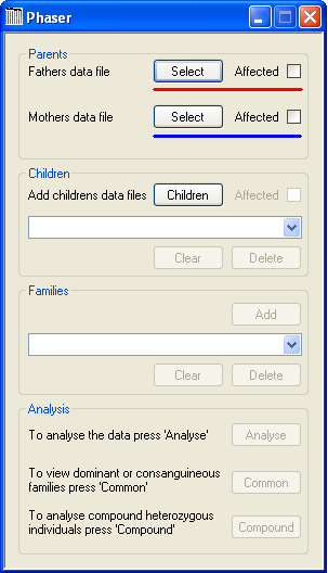
Figure 1
Each family is added sequentially and must include both parents and at least one child (or, if screening for compound heterozygous mutation, at least two children). A parent’s SNP data file is added by using the appropriate button (Figure 1, highlighted in red for a father and blue for a mother). It is also possible to include the disease status of each parent by ticking the box next to each button. The name of the file will then be displayed by the program.
Adding unaffected sibs of affected patients
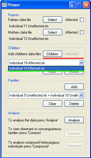
Figure 2
A family must include at least two children when screening for compound heterozygous mutation, or otherwise at least one child. Data for each child is added using the button (underlined in red in Figure 2). After selecting the child’s data file, its disease status is selected via the disease status dialogue form. Typically, each family should include data for affected individuals, unless a 'Shadow Autozygosity MaPping by Linkage Exclusion' project is being undertaken. However, the SAMPLE software is more suitable for the latter type of analysis. When affected children are included, interpretation of results is made easier if the affected children are added before the unaffected children, for each family. The name of the selected data file will be added to the drop-down list (green underlining in Figure 2). To remove a child, select his or her file from this list box and press the button. To remove all children, press the button, which is also located under the drop-down list of children’s filenames.
Data analysis
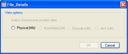
Figure 3
To analyse the SNP genotype data, click the button at the bottom of the main form and choose the unit of distance you wish to use (Figure 3). Only distance units that are present in the data file of the father in the first family can be selected; e.g., in Figure 3 only physical distance is available, since the file contains no genetic map data.
The program will then load the data, first checking for SNPs that have either a “Nocall” genotype or show non-Mendelian inheritance; such SNPs are discarded from the database and any subsequent analysis. Phaser will then reconstruct the chromosomal haplotype of each of the parents in a nuclear family with reference to the genotypes of the first child added to the nuclear family. If other children are included in the family the phase of their chromosomes is deduced by comparing their genotype data to their parents’ haplotypes. By analysing the genotypes of the parents and children it is possible to phase SNPs in all situations except where all of the individuals are heterozygous. When two or more children are included in a family the phase of the majority of SNPs can be found; the number of unphased SNPs is reduced with each additional child added to the family. Unphased SNPs can also be resolved by looking for common haplotypes between members of different nuclear families. While this approach may leave some SNPs unphased, these are more likely to be located in regions where the haplotype is not shared between the different families and so not in the disease-carrying haplotype. In situations where it is not possible to phase a SNP, its genotype will be replaced by a 'C' rather than the usual 'A' or 'B'. Once the SNPs have been phased, those whose genotype conflicts with the parental haplotypes are also discarded.
Viewing the haplotype data
As with AutoSNPa, IBDFinder and SAMPLE, the results are displayed visually and no mathematical or statistical analysis is performed. Rather, the program highlights the movement of large segments of the genome from parent to child, which have undergone relatively few recombination events. The sizes of the fragments that contain the mutant allele are very variable, and the length of a common region consequently does not predict whether or not it contains the disease gene.
It is possible for Phaser to analyse pedigrees for the presence of dominant or recessive disease loci. In the case of recessive conditions, it is possible to analyse both homozygous and compound heterozygous individuals. When screening pedigrees for either a dominant or homozygous recessive disease allele, it is assumed that each nuclear family shares the same mutation as the other families. However, when screening for compound heterozygotes, each nuclear family can have its own pair of disease alleles. To search families for a common disease haplotype (in consanguineous pedigrees or pedigrees with a dominant disease gene), press the button in the Analysis panel. Otherwise, press the button in the Analysis panel (Figure 2).
Identifying common haplotypes in dominant and consanguineous recessive disease families
Pressing the button displays the data window shown in Figure 4. The blue regions show chromosomal segments that have a common haplotype with the selected chromosome. Since SNP data is not present for all regions of a chromosome, the background is coloured white where there are enough SNPs to accurately predict genotype phase (e.g. not around the centromere on Chromosome 1, see Figure 4). If a recombination event occurs, its position is assigned to that of the flanking SNP closest to the q arm telomere.
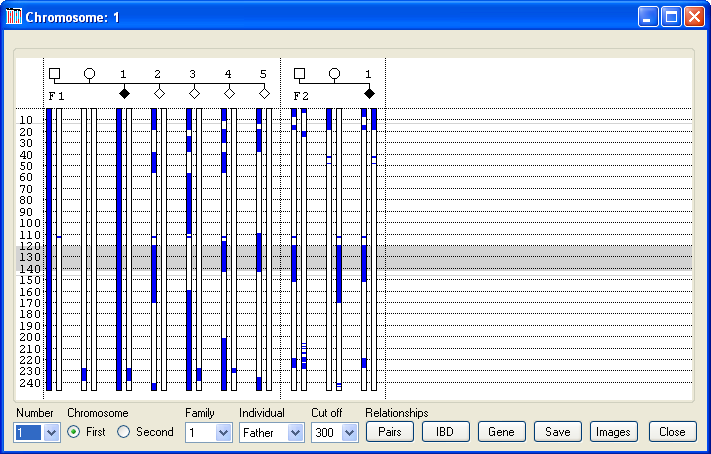
Figure 4
Initially, the first copy of Chromosome 1, belonging to the father of the first family entered, is selected (Figure 4). Phaser always assumes that the first copy of each of the father’s chromosomes is passed on to his first child without any recombination. Similarly, the first copy of each of the mother’s chromosomes is passed on to her first child without any recombination. To change the selected chromosome, select its number from the list box in the lower left corner (red line in Figure 5) and then select either the 'First' or 'Second' option (green line in Figure 5) to pick which of the chromosome homologues to use. To change the individual whose chromosomes are being used as the reference chromosome, first identify the individual’s family in the list box and then the person from the list box (yellow line in Figure 5).

Figure 5
Identifying regions with possible linkage in consanguineous families
In Figure 4, the first chromosome of the father’s Chromosome 1 pair is selected, and so coloured blue along with the first chromosome of the first child. Since this child is homozygous for the disease mutation, it can be assumed that if this chromosome contains the mutation, then the mother will also contain a fragment of this chromosome that is identical by descent (IBD) to this chromosome. Consequently, the part of her chromosome which contains the mutation and is passed on to all affected children will be coloured blue. The only region showing IBD in the parents of the first family is between 230 Mb and 240 Mb. If this region indeed contains the mutation, then all affected children will be homozygous at this position, whereas unaffected children will not. In this case, while the affected child in the first family is homozygous for this region, an unaffected child (child 3) is also homozygous for the common haplotype across this interval, thus excluding this locus. Similarly, the fact that neither parent in the second family has the same haplotype at this point also exculdes this locus. In contrast, if Chromosome 5 is selected (Figure 6), it can be seen that both sets of parents share regions of IBD, as shown by the blue rectangles on their chromosomes. Of these IBD regions, only one, between 121 Mb and 136 Mb, is heterozygous for a common haplotype in both sets of parents. This region is also homozygous in both affected children, while none of the unaffected children is homozygous for this haplotype between 124 Mb and 136 Mb. Subsequent analysis of this interval identified a deleterious mutation in ###### (dotted red line in Figure 6). [To highlight a gene position with a dotted red line, create a tab-delimited text file, with each line containing the gene’s name, the chromosome and the gene’s position (in the same units as the data), as shown in Table 1.
| Name | Chr. | Location | ||
|---|---|---|---|---|
| Gene A | <tab character> | 5 | <tab character> | 126796908 |
| Gene B | <tab character> | 18 | <tab character> | 76456000 |
Table 1
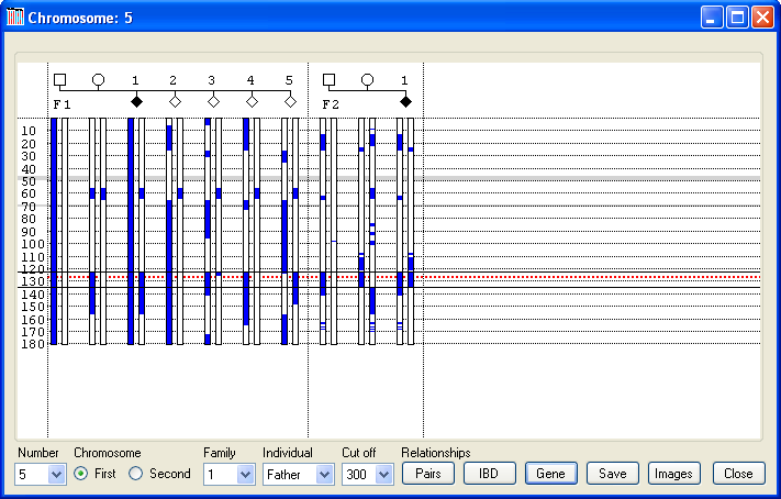
Figure 6
Exporting data
The underlying SNP data can be exported either to a colour-coded web page or to a tab-delimited text file, which can be edited in a spreadsheet program such as Excel. To export data, first select the individual chromosome as described above and then select a region by placing the cursor over the start of the region and pressing the left mouse button (Figure 6). While holding the button down move the cursor to the bottom of the region and release the mouse button. Next press (yellow line in Figure 5), enter the name of the file and select either the *.htm or *.xls file extension to save the data as a web page or tab-delimited text file, respectively.
Example data
In Figure 6, each family has one child affected by the recessive condition early-onset myopathy with respiratory distress and dysphagia (EMARDD). Both affected children are homozygous for a common extended haplotype spanning the region 122– 135 Mb, as shown by the presence of a blue rectangle on each of their chromosomes. All the other children either lack this haplotype or are carriers (like their parents). This haplotype was found to segregate with a frameshift mutation in the MEGF10 gene, which is thus highly likely to be pathogenic change in these families. In Figure 6, the position of MEGF10 is highlighted by the red dotted line at ~126.7 Mb. Examples of exported data for this region can be seen here as a web page or here as a tab-delimited text file. In the web page the genotypes in the common haplotypes are identified by a grey background. In this data set, the MEGF10 gene is flanked by the SNPs RS3097423 and RS7839522. Both file types contain a key which identifies the origin of each chromosome, as well as the phased SNP data. As well as exporting the genotype data from a user-selected region, it is possible to save an overview of the common haplotypes across the entire genome, by pressing the button (blue line in Figure 5). This creates a web page containing images of each chromosome as shown here.Calculating the degree of IBD in each person
Pressing the button (orange line in Figure 5) calculates the level of identity by descent in each person in the dataset. This is done by comparing each chromosome to its homologous chromosome to find regions that have the same haplotype, for runs of at least 300 SNPs. The combined length of these regions is then divided by the entire length of their genome to give a value, where individuals with no common haplotype shared between homologues score 0, while individuals whose chromosome pairs are identical score 1. (The IBD data file for the data used in this guide can be seen here). As with the other exported data files, this file contains a key to identify each person. This data can be used to create a graph of each person’s level of IBD using Excel or other software packages (Figure 7).
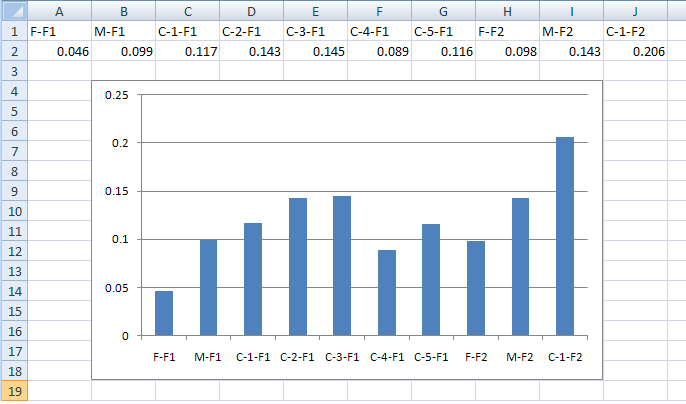
Figure 7
Calculating the degree of relationship between two people
Pressing the button (orange line in Figure 5) calculates the degree of relatedness of each person to the other individuals in the dataset. This is done in a similar way to the IBD calculation, with the length of common haplotypes between the two individuals measured and then divided by the total length of the genome. If a person contains two copies of a shared haplotype (they are homozygous for it) the haplotype is counted twice. This means that if one person is homozygous and the other is heterozygous for a shared haplotype they will score the same for that region as two individuals heterozygous for the same haplotypes. This data is exported to text file which can again be used to create a histogram of the degrees of relatedness between pairs of individuals in a dataset (Figure 8).
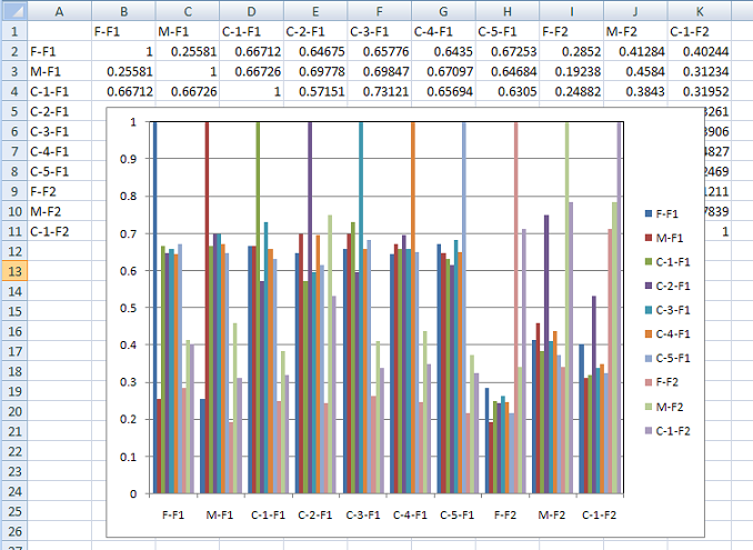
Figure 8
Identifying regions with possible linkage to a disease locus in compound heterozygous individuals
Pressing the button displays the data window shown in Figure 9. This example shows the data for two families affected by cystic fibrosis, known to be caused by mutations in the CFTR gene on Chromosome 7 at 117.2 Mb (red dotted line in Figure 9). In this data set, each of the parents carries a different mutation, and so none of them shares a common haplotype at the disease locus. Like the window shown in Figure 4, regions with no SNP coverage are highlighted as grey horizontal bands. Initially, the window displays the inheritance pattern for Chromosome 1, with a haplotype cut-off length of 300 SNPs. These values can be adjusted using the chromosome and options, as described for the previous window. However, unlike the previous window, the haplotypes inherited from each parent are shown in different colours. The blue regions identify haplotypes identical to those inherited by the first child of the family from its father. Similarly, the pink regions identify regions with the same haplotype as the maternal chromosome inherited by the first child. Since it is assumed that each family in the analysis is not related to the others, each family is analysed in isolation. Therefore a haplotype represented by a blue region in the first family is not linked to the blue haplotype in the second family in Figure 9.
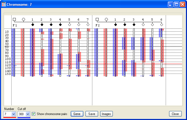
Figure 9
To help explain the process of excluding loci, two regions in Family 1 of the analysis shown in Figure 9 have been highlighted in Figure 10 as pale blue and green bands. Since the first child in this family is affected by a recessive condition, the haplotypes inherited from the child’s mother and father must both contain deleterious mutations. Consequently, Phaser hightlights these alleles as blue (father’s allele) and pink (mother’s allele). If a locus is linked to the disease, then all the affected children should have inherited the same combination of alleles as the first child, which will be displayed in each case as a blue and a pink rectangle spanning the locus. Also, when the alleles of the unaffected children are observed, it would be expected that none of these children share the same combination of alleles as the affected children, and so none of these unaffected children should have both a blue and pink rectangle at the locus. For the region highlighted by the pale blue rectangle in Figure 10, it can be seen that affected children 1, 3 and 4 all share the same maternal and paternal alleles; however child 2 does not, which strongly suggests that this region is not the disease locus. Also, since unaffected child 6 does share both the maternal and paternal alleles, this again strongly suggests that the region is not linked to the disease.
In contrast, within the green region (which contains the causative CFTR gene, the dotted red line in Figure 10), all the affected children share the same combination of paternal and maternal alleles, as seen by the presence of the blue and pink rectangles across the region, while none of the unaffected children share these alleles. This does not prove that this region is the disease locus, but suggests that it is a candidate region. Referring back to Figure 9, it can be seen that the affected, but not the unaffected children in the second family also all share the same paternal and maternal alleles at this locus, supporting its candidacy. In fact, when this process of elimination is repeated for each of the other chromosomes, no other region is consistent with linkage in both families.
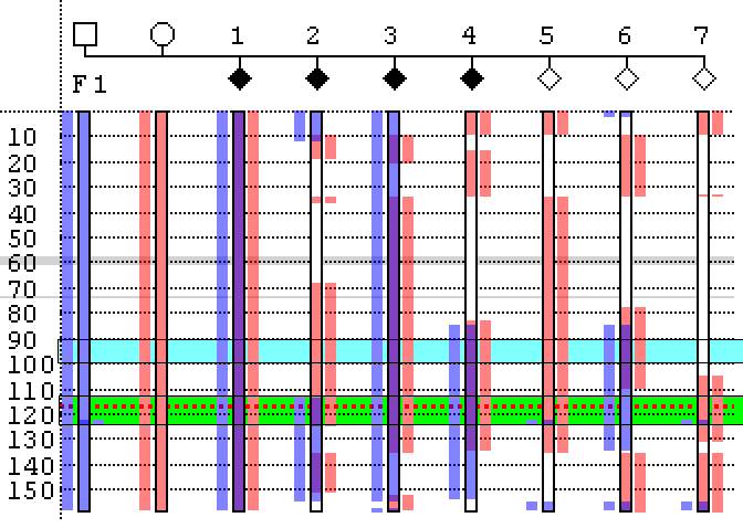
Figure 10
As when performing the haplotype analysis procedure, it is possible to highlight a gene’s position, export the underlying genotype data for a user-selected region, and to create a web page summarizing the inheritance pattern across all the chromosomes. This is done using the , and buttons, as described above for the haplotype procedure. Since it is not expected that families in this type of analysis are inbred, it is not possible to calculate levels of inbreeding via this form.
Exporting data
As when viewing data with a common haplotype, the underlying SNP data can be exported either to a colour-coded web page or to a tab-delimited text file, which can be edited in a spreadsheet program such as Excel. To export data, first select the individual chromosome as described above and then select a region by placing the cursor over the start of the region and pressing the left mouse button (Figure 6). While holding the button down move the cursor to the bottom of the region and release the mouse button. Next press (yellow line in Figure 5), enter the name of the file and select either the *.htm or *.xls file extension to save the data as a web page or tab-delimited text file, respectively.