User guide

AgileVCFMapper was developed using the C# language in Microsoft's .Net Framework 2.0 environment, which is present on all Windows OS's since XP.

Introduction

AgileVCFMapper was developed to duplicate and extend the functions of AutoSNPa and IBDFinder, but using exome variant data in VCF files instead of Affymetrix microarray genotype data. Since the exome data can reasonably be expected to contain the disease causing variant AgileVCFMapper also identifies possible disease causing variants based on the genotype/phenotype of the individuals in the analysis.

As well as visualising the variant data AgileVCFMapper can export the variant data form possible disease loci in VCF files as well as whole genome variant data in a format that can be used other programs published on this site. This feature was included to allow the exome data to be analysed by Phaser, Sample and DominantMapper rather than AutoSNPa and IBDFinder. However, due to the comparatively low variant count in exome data and it's the uneven distribution compared to microarray genotype data, the exome based analysis is not a robust as that achieved using microarray genotype data.

Selecting variant and read depth data

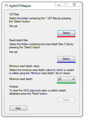
Figure 1: The AgileVCFMapper user interface

The primary source of variant data are the VCF files which list the variants found in each individual in the analysis. These files should be placed in a folder which is selected by pressing the Select button (highlighted by the red line in Figure 1). It is possible for a variant in the database to be absent from a particular individual's VCF, because either the variant is homozygous for the reference sequence or the read depth was too low for the variant calling software to call. Consequently, it may be advantageous to also enter a read depth file for each of the individuals in the analysis. If this is data is available, AgileVCFMapper identifies the read depth for each position for which a variant is present in the analysis as a whole, but absent in an individual's file and updates the variant's total read depth with the value in the read depth file. In subsequent analysis if the total read depth is above the minimum read depth value (described below) the variant is called as homozygous reference. If the read depth is below the minimum read depth value the variant is set to a 'No Call'.

While AgileVCFMapper is designed to function without this read depth data, it is particularly useful when exporting data for use by the other mapping programs as it vastly reduces the number of NoCall genotypes and also allows better detection of de novo mutations (See the 'Detection of de novo mutation detection' section). To enter the read depth data, give each file the same file name as the linked VCF file, appending the '.txt' extension to each file and place them in a folder which can then be selected using the Select button (highlighted by the blue line in Figure 1). The read depth files can be easily generated by GATKLite with the file format shown in Table 1. Since these files may be approximately 1.2 Gbytes each in size reading these file may take several minutes.

Locus	Total_Depth	Average_Depth_sample	Depth_for_2010_0871

chr1:1007177	14	14	14

chr1:1007178	14	14	14

chr1:1007179	14	14	14

chr1:1007180	14	14	14

chr1:1007181	14	14	14

chr1:1007182	15	15	15

Table 1: The format of the optional read depth file. While these files may contain data from a number of samples AgileVCFMapper only read data for a single sample from each file.

Setting the Minimum Read Depth value and call the variant genotypes

The minimum read depth data is set by selecting the desired value from the Minimum read depth data list in the Minimum read depth value panel (underlined by the green line in Figure 1).

When identifying autozygous regions in a patient using exome data, it is often necessary to re-genotype and filters the variants more stringently than the variant calling software used to generate them. Consequently AgileVCFMapper does not take note of the genotype values contained in the VCF file and instead re-genotypes them depending on variants total read depth and the presence of a RS ID value for the variant. It is possible to redefine the minimum total read depth at which a variant accepted using the drop down list (highlighted by the green line in Figure 1). Variants with read depths below this threshold may be not be visualised by AgileVCFMapper, but are still retained by the program and when necessary they will be included in any exported dataset.

Prior experience strongly suggests that variants with an RS ID value are more likely to be genuine variants whereas those without an RS ID value are more likely to be an artefact. Consequently, when a variant does not have an RS ID the minimum read depth value is doubled the selected value. The minimum read depth value may also affect the way in which a variants genotype is deduced, for variants with read depths above the minimum read depth value the genotype is set to:

Homozygous reference: if 80% or more reads contain the reference sequence
Homozygous variant: if 20% or more reads contain the reference sequence
Heterozygous: if between 40% and 60% of reads contain the reference sequence
No Call: if the proportion of reference reads lays outside these values

However, if the read depth is less than the minimum value, but greater than half the minimum value the variant genotype is set to:

Homozygous reference: if 80% or more reads contain the reference sequence.
Homozygous variant: if 20% or more reads contain the reference sequence
No Call: if the proportion of reference reads lays outside these values

Once the location of the VCF files and the optional read depth files has been selected the data is imported and processed by pressing the Read button in the Analyse panel at the bottom of the window. Initially, the VCF files are read and used to create a variant database. Once the database has been created the optional read depth files are read and the data added to the variants not present in an individual's VCF file. The name of the file that is currently been processed is shown next to the appropriate Select button and when the processing is completed the Analysis methods window appears (Figure 2).

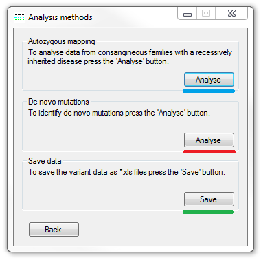
Figure 2: The Analysis methods window.

Visualising the variant data

The Analysis methods window (Figure 2) allows the selection the desired analysis pathway. These consist of visualising the data to aid either the identification of common autozygous regions or identify variants with a non-Mendelian inheritance pattern that may suggest the presence of de novo mutations. This window also allows the variant data in the variant database to be exported to tab-delimit files that can be used in other mapping software applications. A comparison between using exome and microarray derived variant data to map an disease locus in an out-bred family using PHASER can be found here.

While the windows used to display the data for autozygosity mapping or de novo mutational analysis differ they both contain a number of common feathers which will be discussed prior to describing how to use each form.

Common features of the variant data displays

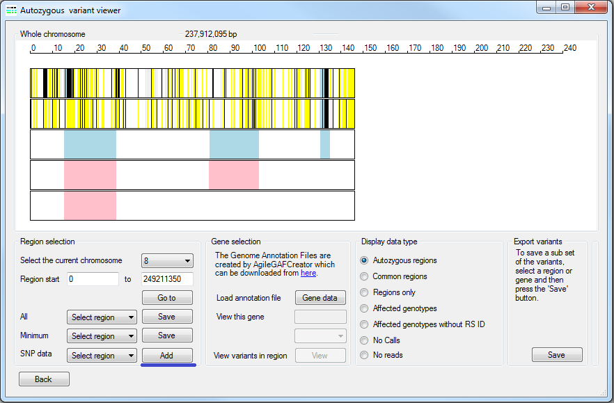
Figure 3: Generic functions of the analysis windows of AgileVCFMapper

Both windows are composed of two regions; the upper half displays the variant data, while the lower half contains the data display options (Figure 3). Initially, the variant data for the entire length of chromosome 1 is displayed, with the data for each individual arranged as a horizontal strip of colour coded vertical lines. The colour coding varies depending on the display option selected in the Display data type panel.

The origin of each row of data can be determined by placing the mouse cursor other the data and causing the file's name to be displayed in the top right of the data view (see the blue rectangle in Figure 4 A). The location of the cursor, relative to the chromosome, is also displayed above the display view (see the red rectangle in Figure 4 A).

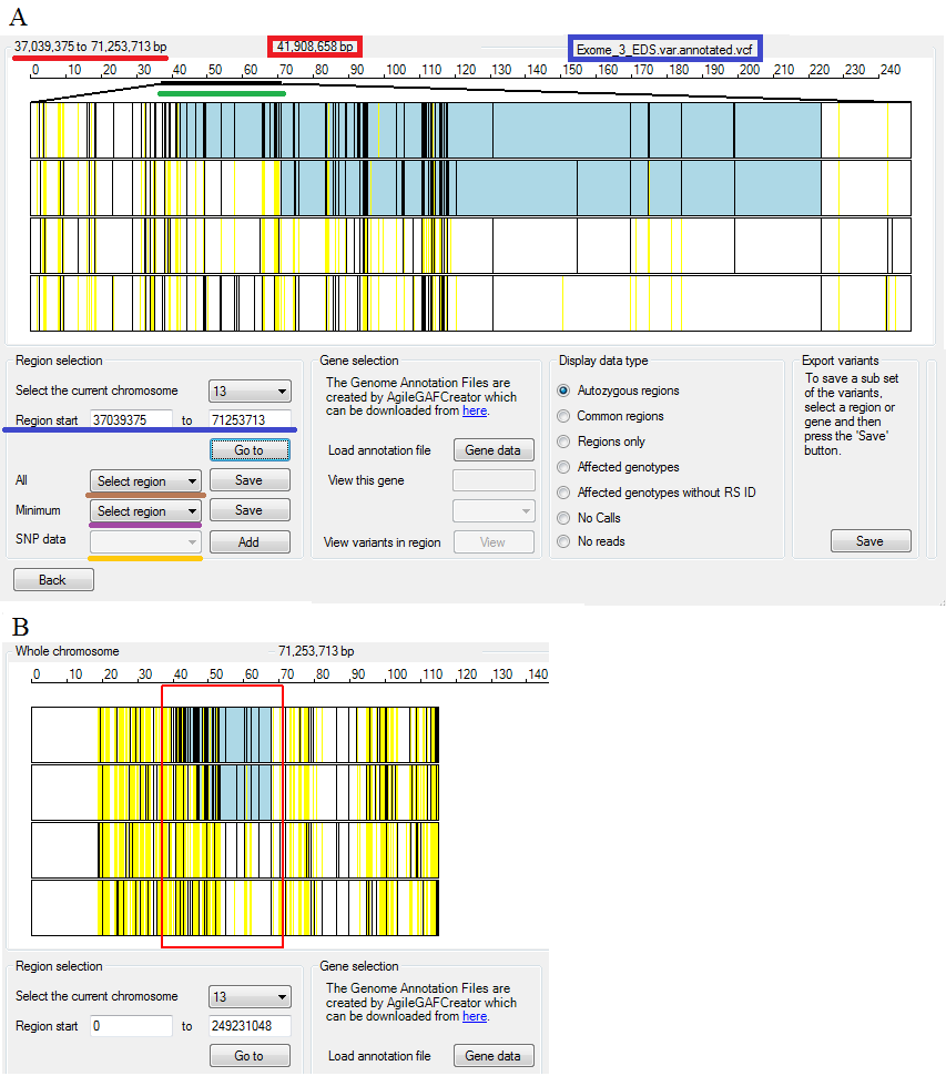
Figure 4: Navigation of and user feedback of the variant display region

Selecting a chromosomal region

The Region selection panel on the left of the lower options region allows the selection specific parts of a chromosome. To change the currently displayed chromosome, simply select the chromosome's number from the drop down list in the top of the Region selection (underlined by the blue line in Figure 4 A and B). When a chromosome is selected, variant data is displayed to the same scale as the longest chromosome in the data set. Initially this is defined by the variants in the VCF files with a chromosome's length taken as the position of the last variant plus 0.1 M bases.

It is possible to zoom in on a region by either entering the regions co-ordinates or by selecting a region with the mouse.

To select a region using its co-ordinates enter the base pair positions delimiting the region in to the text boxes below the chromosome selection drop down list (underlined by the blue line in Figure 4 A and B) and then press the Go to button.
To select a region using the mouse, move the mouse cursor to the start of the region and hold down the left mouse button while moving the cursor the end of the region. The selected region will be shown by a red rectangle (Figure 4 B). When the mouse button is released the display will zoom in to the selected region (Figure 4 A).

The base pair co-ordinates delimiting the visible region are displayed at the top left of the variant display region (underlined by the red line in Figure 4 A), while the regions relative location on the chromosome is shown by a black line (underlined by the green line in Figure 4 A). The region's location is also displayed in the Region selection panel irrespective of how the region was selected (underlined by the blue lines in Figure 4 A and B). To view an entire chromosome either click on the variant display image or re-select the chromosome from the drop down list.

Viewing annotated variant data relative to gene's sequence

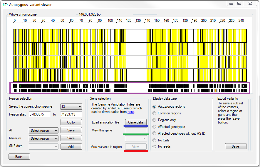
Figure 5: Entering gene data and viewing variant data with reference to the gene data

AgileVCFMapper can display the variant data with reference to their position a gene. This enables the rapid detection of putative disease causing variants in known disease genes or strong functional candidate genes. To import the required gene information, press the Gene data button in the Gene selection panel and select a *.gaf file (underlined by the blue line in Figure 5). These files can be created by AgileGAFCreator which can be found here. These files contain the sequence and genomic co-ordinated for all the exons in genes annotated in the CCDS or RefGene data sets. Once imported, the location of the genes on the current chromosome will be shown below the variant data (violet box in Figure 5). The genes are drawn as a series of black rectangles in which the exons of genes on the forward strand are coloured green while those on the reverse strand are coloured orange (Figure 5).

It is possible to select a gene by clicking on it using the mouse, selecting its name from the list box file or typing its name in to the text box below the Gene data button (see the green rectangle in Figure 5). The list box automatically contains the names of the genes in the currently displayed region. Selecting a name from this list, will automatically cause the display to zoom into the gene's position (which will be highlighted by a red rectangle) along with flanking sequence. This allows the presence of variants in the gene can be rapidly determined (Figure 6). It is also possible to select a gene by directly typing the gene's name in to the text box above the gene list with this method allowing the selection of a gene anywhere in the genome and not just the currently selected region. By using this feature it is possible to rapidly search a list of known disease genes to identify those in autozygous regions and with possible disease causing variants.

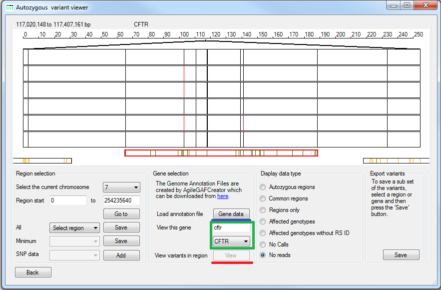
Figure 6: Viewing variant data with reference to a gene

The Variant Viewer window

By pressing the View button in the Gene selection panel (underlined by the red line in Figure 6) it is possible to view in depth information for each of the variants in the currently selected region on a gene by gene basis (Figure 7). This function is only available when displaying using the Autozygous regions, Common regions, Affected genotypes and Affected genotypes without RS ID options on the Autozygous form and all options on the De novo mutations window. When used with the Autozygous regions and Common regions display options all variants in the currently selected region are included irrespective of whether the variants are displayed or not, however, when used with the other display options only the variants that are displayed are included in the Variant viewer variant list.

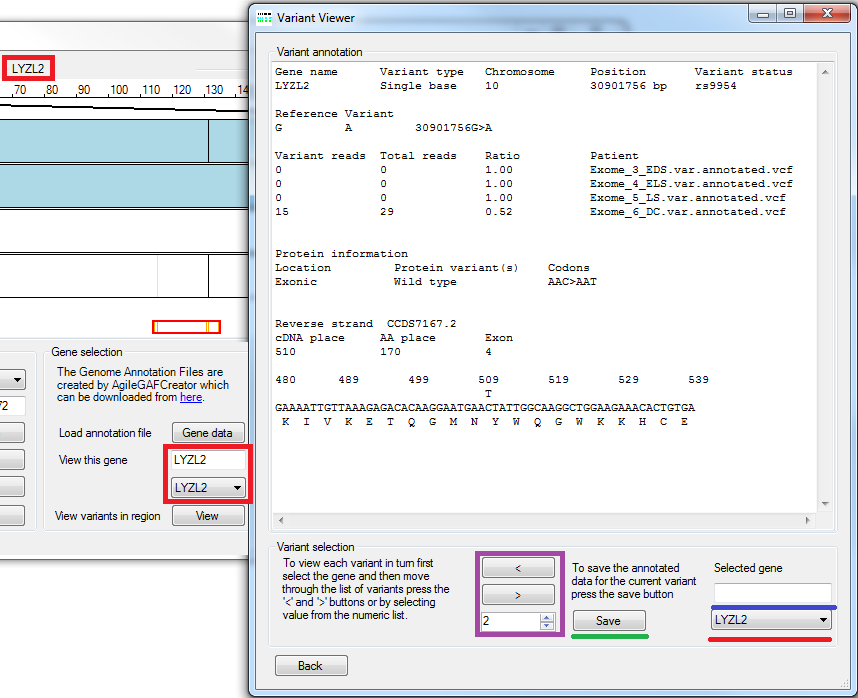
Figure 7: Viewing variant data in a gene

To view variants in a gene either select its name from the list of gene names in the bottom right of the window (under lined by a red line in Figure 7) or type the gene's name in to the text box above this list (under lined by a blue line in Figure 7). Once selected the display in the 'parent' window will zoom in to the gene and the large text box in the Variant Viewer window will contain information on the first variant in the gene (The variants are ordered by chromosomal location and not 5' to 3' in the selected gene). If the gene contains more than one variant, it is possible to iterate through the list of variants using either the '<' or '>' buttons or the number list box control (in the violet rectangle in Figure 7). The genotypes of the variants are not displayed in the variant annotation text; instead the variant's read and total read depths are shown so the user can discern the variant's genotype themselves. It is possible to save the variant annotation text by pressing the Save button (under lined by a green line in Figure 7).

Autozygous variant viewer window overview

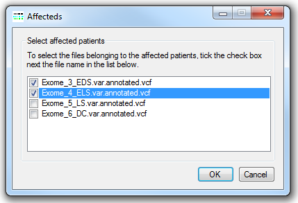
Figure 8: Identifying data from the affected patients

To analyse the variant data for common autozygous regions press the Analyse button in the Autozygous mapping panel (highlighted by the blue line in figure 2). Before the data is visualised it is necessary to identify which of the VCF files originates from an affected individual, consequently having pressed the Analyse button the Affected window is displayed (Figure 8). This window contains a list of the filenames in the analysis. To identify a file as originating from an affected individual tick the check box to the left of the file's name. Once all the affected individuals have been selected, press the OK button, this will close the Affecteds window and open the Autozygous variant viewer window (Figure 9).

Figure 9: The Autozygous variant viewer window displaying variant data derived from exome data (upper to rows) and Affymetrix microarray SNP genotype data (lower three rows).

AgileVCFMapper contains an automated function that identifies autozygous regions in each individual. These autozygous regions are displayed as either pale blue rectangles for affected patients or pink rectangles for unaffected individuals (Figure 10) and are always displayed irrespective of the currently selected data display option. A comparison of the autozygous regions identified using exome data and microarray SNP genotype data can be seen here. If SNP microarray genotype data is available for family members, it is possible to include this data in an analysis by placing the genotype data files in an empty folder and selecting it by pressing the Add button (underlined by the blue line in Figure 9). AgileVCFMapper can read data formated as the original *.xls or newer birdseed text files.

Selecting a chromosomal region corresponding to a predetermined autozygous region

As well as the options described above, the Region selection panel contains two extra dropdown lists which contain the co-ordinates of the autozygous regions identified in the affected patients. The upper list (underlined by the brown line in Figure 10 A) contains all of the regions in the affected patients, while the lower list (underlined by the violent line in Figure 10 A) contains regions that are present in all the affected patients. It is important to note that these regions may also be present in unaffected individuals and are not necessarily concordant among the affected patients. Selecting a region automatically updates the values in the other options in the Region selection panel and zooms in to the selected region. It is possible to save the lists of regions in each drop down list to a text file by pressing the Save button to the right of the appropriate control.

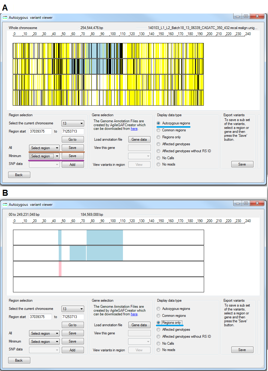
Figure 10: The Regions and Autozygous regions options

Displaying variant data to suite different mapping approaches

Identification of disease loci in unrelated consanguineous individuals

using the Regions and Autozygous regions options

This pair of display options duplicates the mapping approach used IBDFinder which maps disease loci using microarray SNP genotyping data from unrelated individuals with the same disease phenotype.

AgileVCFMapper can display the location of autozygous regions with or without displaying the underlying variant data by selecting either the Autozygous regions or Regions only options respectively (Figure 10 A and B). As stated earlier autozygous regions in affected patients are shown as blue rectangles, while the rectangles in unaffected individuals are drawn in pink. When viewed with variant data the variants are shown as colour coded vertical lines with homozygous variants drawn as black vertical lines, heterozygous genotypes are shown as yellow lines and NoCall genotypes are not displayed at all. Where two different variants are located to the same pixel in the image, heterozygous genotypes are displayed in preference to homozygous genotypes. Viewing the data without the variant data can be particularly useful when identifying short regions which may be obscured by the variant data such as the region at 45 Mb in figure 10.

Note: It is important to realise that these regions are identified only using variants associated with an RS IDs in the VCF files. If these files do not contain RS ID any regions will not be displayed!

Exome data may contain a high proportion of miss-called genotypes compared to microarray SNP genotype data. Consequently, when verifying the autozygous regions it is helpful when zooming in on the region to also include the flanking regions and compare the variants in the autozygous region to those around it. Typically, the autozygous region will have noticeably less yellow lines than the flanking region (Figure 11).

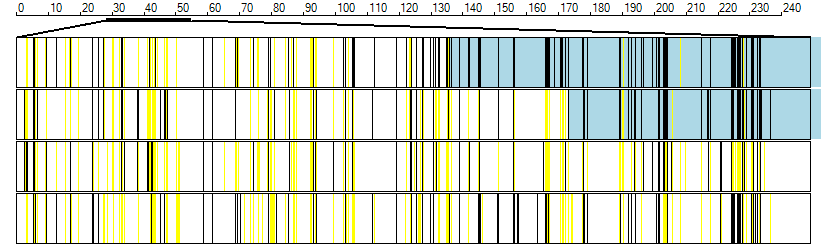
Figure 11: When viewing an autozygous region it may be helpful to first view the region with flanking sequence to correctly delimit the regions.

Identification of disease loci in related consanguineous individuals

Using the Common regions, affected genotypes and affected genotypes without RS ID options

These display options duplicates the mapping approach used AutoSNPa which maps disease loci using microarray SNP genotyping data using related individuals in which the disease allele is the same in all affected patients.

AgileVCFMapper is also able to aid the identification of autozygous regions that are concordant among the affected patients, but not unaffected individuals. It is very important to note that this analysis is best performed with data that includes the read depth data so that homozygous reference variants can be effectively distinguished from positions with a No Call genotype due to low read depth. If no read depth data is used the display for the Common regions option may be indistinguishable from the Autozygous regions display described above.

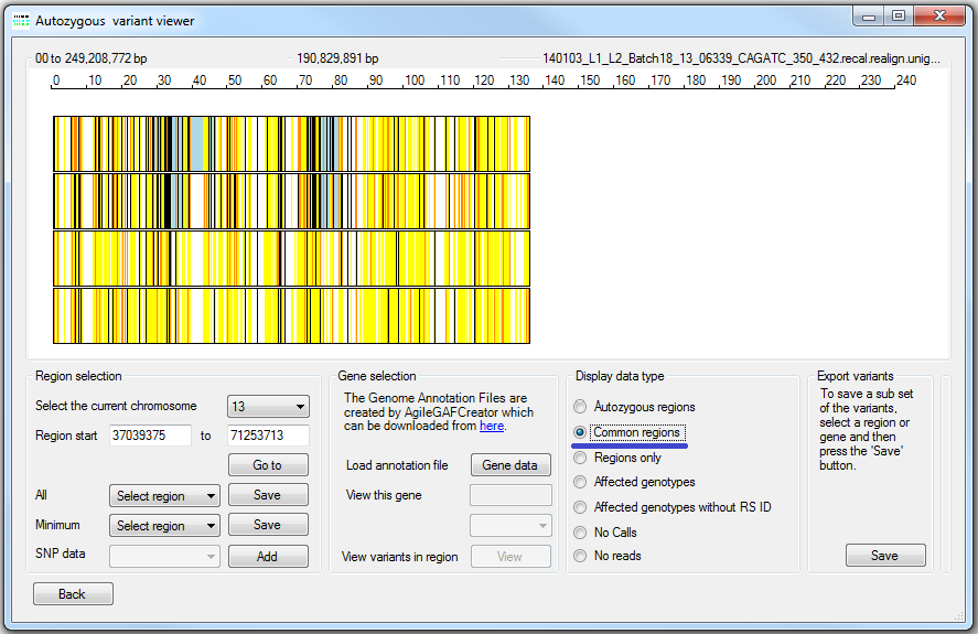
Figure 12: The Autozygous regions option.

Concordant regions are viewed by selecting the Common regions option (underlined by the blue line in Figure 12). Autozygous regions are drawn as blue or pink rectangles as described earlier and the variants are drawn as colour coded vertical lines. If all the affected patients are homozygous for the same allele the variant is displayed as a black line, otherwise the variant is drawn as a yellow line, while uncalled genotypes (No Calls} are not displayed. Since the resolution of the image is small compared to the size of a chromosome, a number of variants may be placed at the same point on the image. If more than 20% of the variants mapped to the same point are to be drawn as yellow lines then a yellow mark is placed at that position. If more than 90% of the variants at the same point on the image are to be drawn as black lines, then the position is marked with a black line. For positions which fall between these two cut offs, the location is marked with a grey line. Figure 13 shows a comparison for the displays generated by the Regions Only, Autozygous regions and Common regions options for an autozygosity region that is not concordant in the affected patients. It can be seen that the number of black vertical markers is higher in the autozygous regions display (Figure 13 B) than the Common regions view (Figure 13 C) showing that the regions are autozygous but not for the same haplotype (highlighted by the red line).

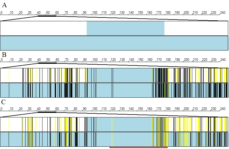
Figure 13: A comparison of the Regions Only, Autozygous regions and Common regions options.

Since the analysis is based on sequence variants in the genomes of the affected patients and their relatives, the analysis should contain the disease causing. Consequently, it is possible to filter the variants for genotypes that are homozygous variant in all the patients but not homozygous variant in any of the unaffected relatives. The results of this analysis can be filtered further by only viewing variants which do not have an RS ID value, which should be absent form novel variants that cause rare recessive diseases but may be present in conditions where disease causing variants have previously been published. Variants which are homozygous non-wildtype in the patients, but not their relatives are visualised by selecting the Affected genotypes option (highlighted by the blue line in Figure 14 A), while variants which also lack a RS ID can be seen by selecting the Affected genotypes without RS ID option (highlighted by the red line in Figure 14 B).

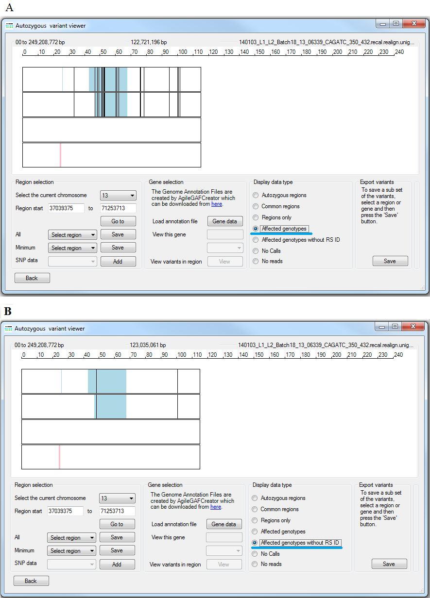
Figure 14: A comparison of the Affected genotypes and the Affected genotypes without RS ID options.

Displaying regions of poor coverage and No Calls

Using the No Calls and No reads options

Since the variant data sets may contain a variable level of variants with 'No call' genotypes, it is possible to view variants that have a 'No call' genotype. The No reads options displays variants as red lines if the read depth is below the read depth cut off value, otherwise the variant is shown as a black line. If variants map to the same point on the display image, variants with low read depths are shown in preference to those with higher read depth. Consequently it is normally necessary to zoom in on a region to fully understand the number of variants that have low read depths. Similarly, the No Calls options identifies variants that do not have a genotype because they have either a low read depth or the ratio of variants reads to reference reads is not a value expected from a diploid genome. Figure 15 shows a series of images from the PMS2 locus which spans a highly homologous duplication and so contains variants with allele read depth ratios that differs from the expected values due to problems aligning the reads to the correct sequence in the duplication. Figures 15 A and B shows the data display for the No Reads option when variant data is entered without and with the optional read depth data respectively. The red lines identify variants heterozygous or homozygous for the variant sequence whose total read depth is below the 'Minimum read depth value' or variants homozygous for the reference sequence and so not included in the VCF files. By importing the read depth from an optional read depth file the number of variant's with no reads (read lines) is reduced as the read depth of homozygous reference sequence positions are now known.

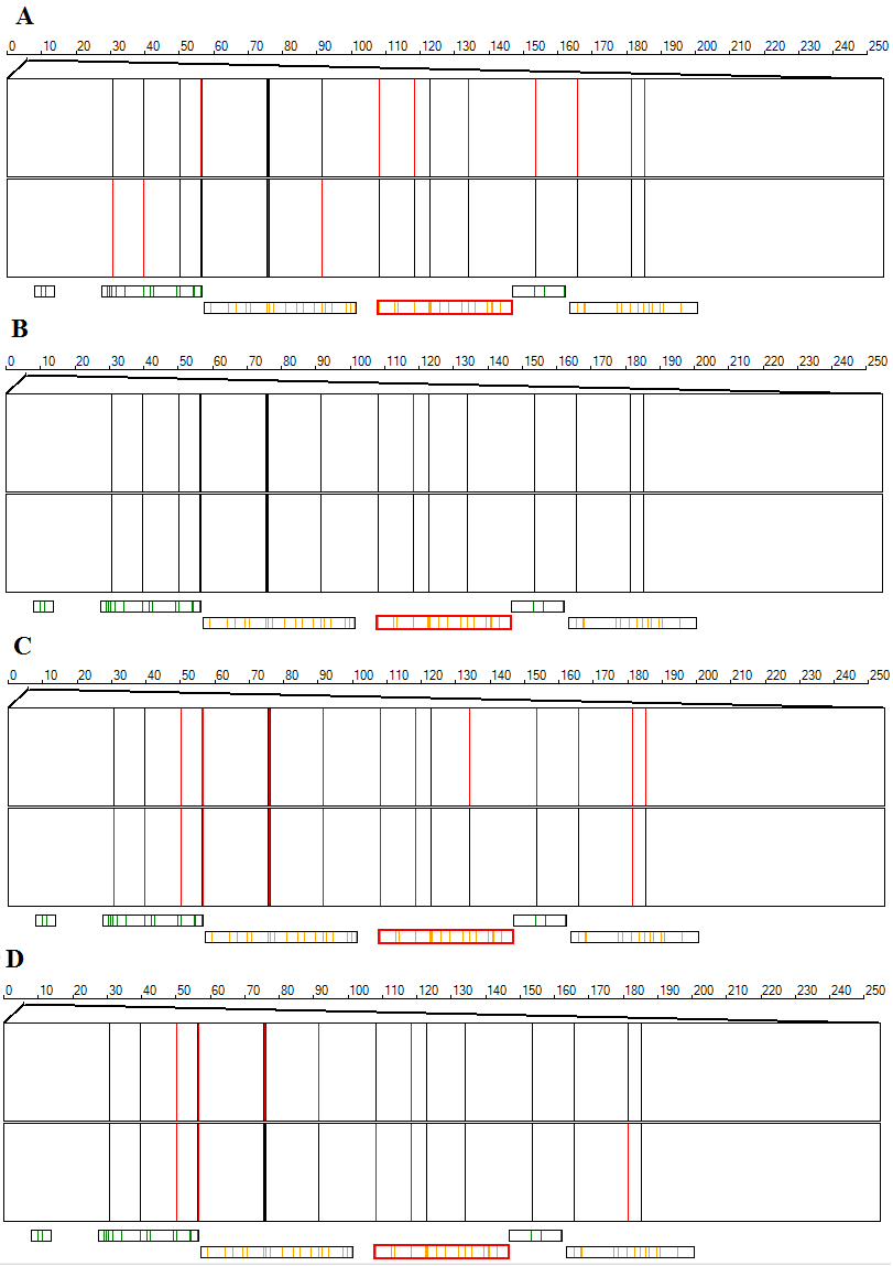
Figure 15: A comparison of the No Calls and No reads options with and without the optional read depth data.

Similarly Figure 15 C and D show the display generated by the No Calls option without and with the optional read depth data. Variants with a 'No Call' genotype are shown as a red line, whereas variants with a genotype are shown as a black line. This display produces a similar image to the No Reads option; variants with a read depth about the minimum cut off may be ascribed a 'No Call' genotype if the allele read depth ratio is not in the value range expected for a diploid genome. Since the region shown in Figure 15 contains the PMS2 duplication a noticeable proportion of the variants receive a 'No Call' genotype. If a variant's read depth is greater than half the minimum read depth value, but less than this cut off it may still be scored as a homozygous genotype if more than 80% of the reads belong to a single allele. Consequently, variant's that are shown as red lines in the No Reads display may appear as black lines in the No Calls display.

Exporting variants from the selected region

It is possible to sequentially export variants from selected regions by selecting a region and then pressing the Save button. This will produce a VCF file that contains all unfiltered variants in the selected regions. This function does not utilise the data in the variant database used to create display images, instead it re-reads the original VCF files and copies the appropriate variants to the new file. Consequently, the original data format is maintained in the new files which can then be used in other exome variant analysis programs.

De Novo mutation detection

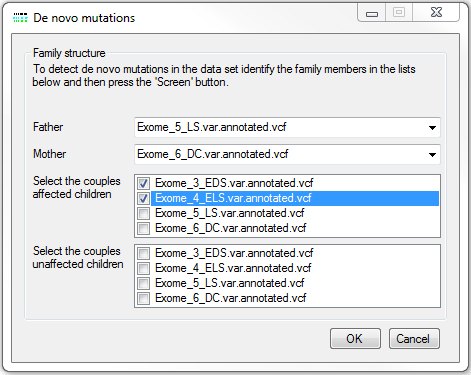
Figure 16: The De novo mutations window allows the different members of the family to be identified.

If a study contains exome data from a nuclear family consisting of both parents and a number of affected children it is possible to screen the variant data for instances of non-Mendelian inheritance. This is performed by pressing the Analyse button on the De novo mutations panel of the Analysis methods window. This causes the window in Figure 16 to be displayed, which contains four lists of the files in the current analysis. The first two lists are used to select the data derived from the father and mother, while the last two lists are used to select the data from the affected and unaffected siblings. Once the origin of the files has been set, pressing the Ok button closes this window and opens the De novo variant viewer window (Figure 17). Many of the functions in this form have been described at the start of this user guide in the 'Common features of the variant data displays' section, with only the functions in Display data type and Export variants panel containing new functions. As before the Display data type panel contains the functions that control how the data is displayed. It is possible to exclude all variants from the display that are linked to and RS ID by ticking the Exclude variants with RS ids check box (under lined by a blue line in Figure 17). A variant is only shown as a possible de novo mutation if both parents have a genotype ascribed to the variant and all the affected children show the same possible variant, while none of the unaffected sibling shows a non-Mendelian inheritance pattern. This means that if multiple affected siblings are in the analysis, only a single affected child may show a non-Mendelian inheritance pattern, but all the affected siblings have a genotype consist with them inheriting the de novo mutation.

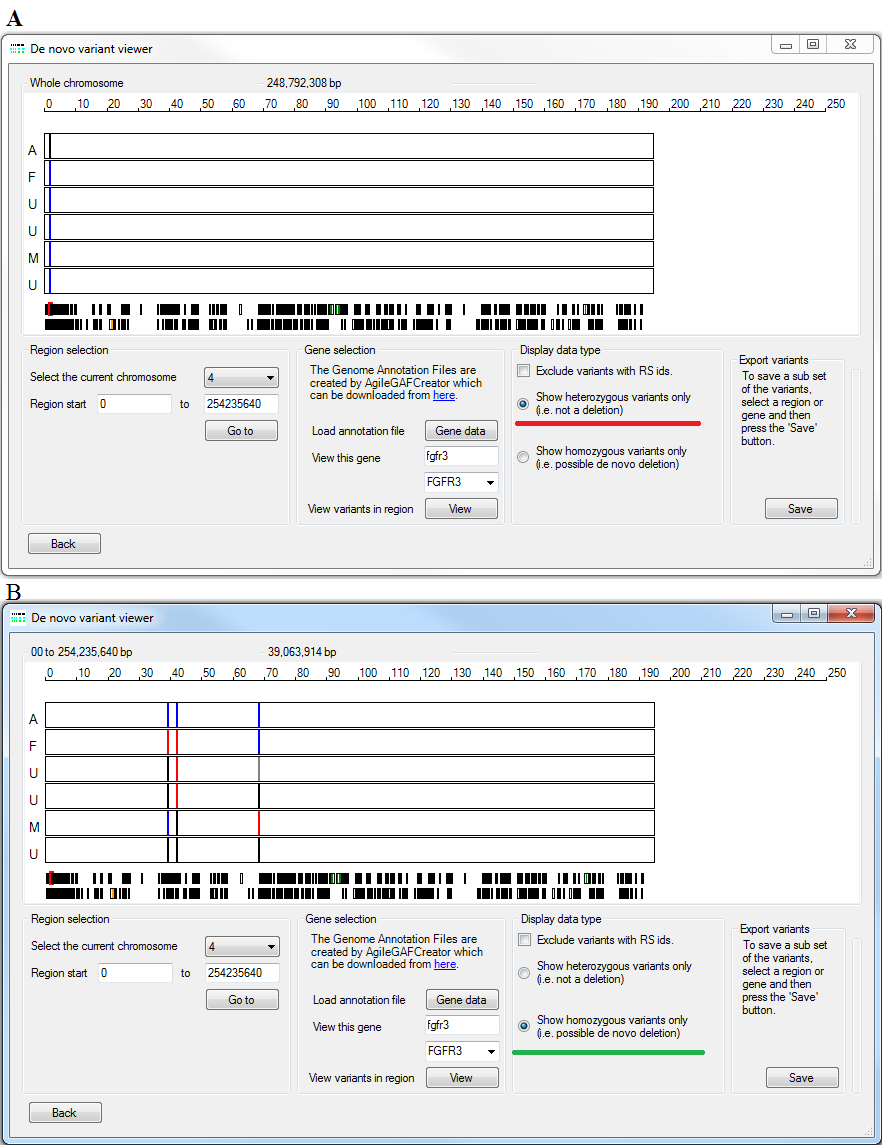
Figure 17: A comparison of the Show heterozygous variants only (i.e. not a deletion) and Show homozygous variants only (i.e. possible de novo deletion) options.

De novo mutations typically appear as either variants that are heterozygous, but are expected to be homozygous, or homozygous variants that should be heterozygous. Consequently, it is possible to view de novo mutation that result in individuals with an unexpected heterozygous or homozygous genotype, by selecting the Show heterozygous variants only (i.e. not a deletion) or Show homozygous variants only (i.e. possible de novo deletion) options (under lined by the red and green lines respectively in Figure 17 A and B). In each view the genotypes of the variants are called codes with homozygous reference sequence variants drawn in blue, homozygous variant sequence variants drawn in red and heterozygous variants drawn in black, while variants with an uncalled genotype shown as a grey line. If more than one variant is mapped to the same point on the image the genotypes of the last variant are shown.

Exporting data

Pressing the Save button saves the variants currently visible in the variant display region. The variants are saved as to a tab-delimited text file which contains the variants position, alleles and the genotype data and read depths for each of the individuals in the analysis. The variants export file's structure is shown in table 2.

RS name	Chromosome	Position	Reference	Alternative	Parent1.vcf	Ref\|Alt read depth	Parent2.vcf	Ref\|Alt read depth	Affected.vcf	Ref/Alt read depth
rs2273311	1	16641899	C	T	C:C	85\|0	C:C	61\|0	C:T	47\|47
rs9435793	1	17265560	C	T	C:C	15\|0	C:C	15\|3	C:T	19\|13
-	1	17292223	G	A	G:G	26\|0	G:G	20\|0	G:A	19\|17
rs12059633	1	17292404	A	G	A:A	90\|0	A:A	61\|0	A:G	71\|60

Table 2: The structure of the file containing information for variants with a non-Mendelian inheritance pattern suggesting de novo mutations.