Walk-through user guide
Table of Contents
1.1 Before running the program
1.3 Selecting a sequence variant for analysis
1.4 Setting the analysis options
2.1 The *.xls tab-delimited text file
3.3 Selection of sequence variant
– Appendix—effect of varying reference peak selection
1 Analysing data
1.1 Before running the program
We use the term "QSV" (quantitative sequence variant) throughout this guide, to refer to any site where two sequence variants are superimposed in a sequence trace. These may be allelic (i.e. the QSV is a SNP, and the expected allelic proportions are 0.5, 0.5). More generally, though, the QSV is composed of contributions from allelic and/or paralogous DNA sequences, whose copy number may not be known.
All the sequence trace files to be analysed must first be placed in a single folder. Note that with some security settings, the Windows XP or Vista operating system may block the program from accessing files located in a network folder. Similarly, the program itself may be blocked from running from a network folder. To avoid these problems, copy both the data folder and the executable program file (QSVanalyser.exe) to a location on a local drive.
1.2 Viewing a trace file
The initial program interface is shown in Figure 1. To open a sequence file, select > . This menu allows the user to select *.scf, as well as ABI and Megabace trace files.
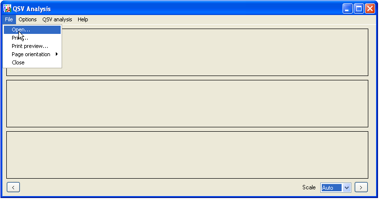
Figure 1: The File menu contains the Open option as well as the Print functions.
Once opened, a file’s nucleotide sequence and trace are displayed as shown in Figure 2. The peak height scaling can be adjusted using the list-box (Figure 2, blue ellipse). Its default value of Auto adjusts the tallest peak height to fit the height of the display panel. This may cause unwanted flattening of some sequences if they contain very large peaks (due to dye blobs or other sequencing artefacts), but can be overridden by manually selecting a new scale value. The two corner buttons (green ellipses) are used to navigate along the DNA sequence, the left () and right () buttons moving to a position in the sequence 5′ and 3′ of the current position, respectively. Since the program is designed for analysing heterozygous or superimposed paralogous sequences, it will display IUPAC ambiguity codes, e.g. R (A+G), W (A+T), S (C+G) and Y (C+T), although only if the peaks representing the two variants are comparable in height.
The trace numbering (Figure 2, red ellipse) can be changed via the > menu to show either the sequencer scan number (default), the base pair number or no labels at all. The menu also contains the menu, which displays the average peak height values, either as text or as a horizontal line on the display panels.
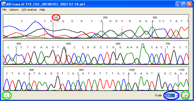
Figure 2: Electropherogram data displayed by QSVanalyser.
1.3 Selecting a sequence variant for analysis
A sequence variant can be entered using the keyboard, selected from the current electropherogram, or imported from a file. To select a variant from the current sequence trace, tick the menu item and then left-click with the mouse pointer over the desired sequence variant, as shown in Figure 3.
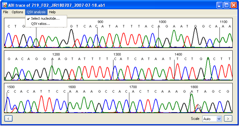
Figure 3: To select a variant from the current file, tick the Select nucleotide… menu item and then click the left mouse button over the desired peaks on the display panel.
Otherwise, select the > option. Ultimately, the form shown in Figure 4 will be displayed. If you chose the option, the sequence data should already be entered.
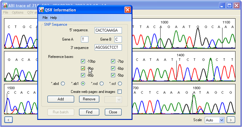
Figure 4: The QSV information form allows the user to enter the variant’s sequence and analysis options.
The first four input fields of the QSV information form allow the user to enter or edit the 5′ and 3′ flanking sequences (10 nt), define the sequence variant itself, and select the order in which the variant nucleotides will be placed in the analysis output file. Only the four standard bases (A, C, G and T) should be entered here; ambiguity codes (e.g. R, S, W, or Y) will not be analysed correctly. To check the entered sequence information, press the button. Provided the entered sequence is correct, a new QSV image window will appear, showing the current sequence trace around the chosen QSV (Figure 5). If the sequence variant data have been entered incorrectly, an error message will be shown. When the QSV image window is closed the QSV information form will reappear.
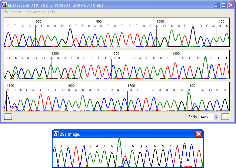
Figure 5: Pressing the Find button on the QSV information form (Figure 4) scans the current trace file for the desired variant, and if found, displays an image of the trace data.
1.4 Setting the analysis options
When the program analyses each trace, it adjusts the QSV peak heights relative to the peak heights of upstream nucleotides. These are user-selectable, via the six checkboxes below the Reference bases label. If more than one reference nucleotide is selected, the QSV will be scaled relative to the average height of the selected reference peaks. Initially, it is recommended that all six reference positions are selected, and the data analysed with the option selected (see below); this will create a web page (see the Web page structure section) containing information on the variability of these nucleotides (and so identify bases that are unsuitable for use as reference peaks). For a more detailed example of the effect of reference peak choice, see this page.
The type of trace file to be analysed is selected via the radio buttons below the checkboxes. Only one type of file can be analysed per batch. Selecting the option creates a web page containing images of the sequence around the QSV, plus peak height information for each trace file. The structure of this file is explained in more detail in the Web page structure section. Since the production of a web page involves the creation of multiple trace images, selection of this option slows the analysis significantly. (This overhead results from the time required to save the images to disk, and is largely independent of the speed of the computer’s processor.) Nonetheless, it is recommended to create a web page until the user is confident that each variant is analysed correctly.
After checking that the program can find the specified QSV in the current file, that variant can be imported by pressing the button. This will store the sequences and the selected reference peaks. If two or more QSVs are to be screened per PCR product, the process can be repeated for each QSV. QSVs can be viewed by selecting them using the list-box next to the and buttons. To edit a QSV, change its options and press the button; note that this will result in duplicate data for that QSV. If you do not wish to analyse the QSV with multiple options, select the original and delete it using the button.
If the same QSVs are to be analysed repeatedly, it is possible to save the QSV and selected reference peak specifications to a text file, which can then be used to re-enter the data. This is done via the > and > menus on the QSV information form.
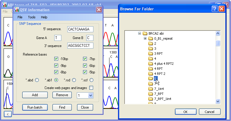
Figure 6: To analyse the data press the Run batch button and select the folder containing the trace files.
1.5 Analysing the data
Once the analysis options have been set, the analysis can be started by pressing the button on the QSV information form. The user will be prompted to select the folder containing the trace files (Figure 6). The QSV information form will close and the program will analyse all the trace files in the folder. The results are exported to a subfolder named QSV_data within the trace files folder (Figure 7). If this folder does not already exist, it will be created, while if it does exist, any files from a previous analysis may be overwritten. To prevent this, rename either the results folder or its individual files. The peak height data are always saved to a single tab-delimited text file with a *.xls file extension. In addition, if the Create web pages and images option is selected, data for each variant are also saved to a web page.
During analysis, the name of the file currently being analysed will appear in the program’s title bar. However, the program may appear to stop responding, since to expedite analysis the program will not refresh its appearance. When the analysis is complete, a message box will appear, identifying which trace file is currently displayed by the program. Since the program analyses each file independently of other traces, it can screen in excess of 1250 files per run (using Windows XP, P4 3.2GHz and 1GB of RAM). However, it is recommended normally to run the analysis on a per PCR plate basis (96 or 384 samples).
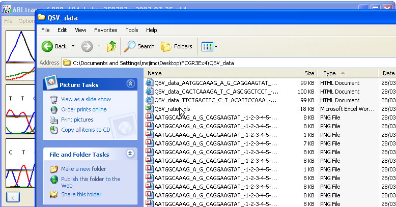
Figure 7: The output files are saved to a subfolder called QSV_data
2 Output data files
The program creates two types of output; a tab delimited text file with a *.xls file extension, and optional web pages, each comprising one *.htm file and a collection of *.png image files. Each analysis creates a single *.xls file, while each variant analysed creates a separate web page, if the option is selected.
2.1 The *.xls tab-delimited text file
This file contains the name of the trace file, adjusted peak heights for each variant, the proportion of the peak heights (adjusted peak height of variant A ÷ sum of the peak heights of variants A and B) and the average intensity of the reference nucleotide peaks. If more than one variant is analysed, these columns are repeated (Figure 8). The final column shows the average peak height ratio for all of the variants screened in a file. At the bottom of the file, the mean intensity of the reference peaks (i.e. the value in column E of Figure 8) for each variant, and its standard deviation are shown. These data are included to help identify batches with a high level of intra-assay variation.
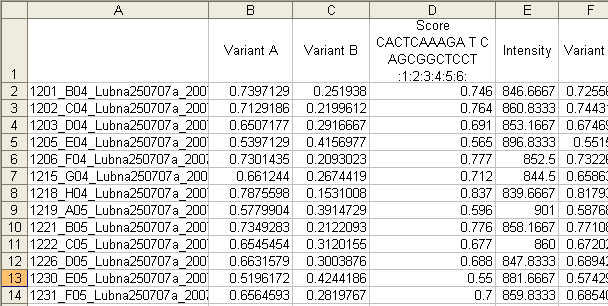
Figure 8: The tab-delimited text output file is best viewed in a spreadsheet application. The columns contain the following data: (A) file name, (B) variant A peak height, (C) variant B peak height, (D) peak height ratio and (E) reference peak average intensity.
2.2 Web page structure
If the option was selected, a web page is created for each QSV. This page has three sections; the first section contains a table showing the trace image around the QSV and the relative peak height data for each of the nucleotides in the surrounding sequence as well as the variant peak heights (Figure 9).
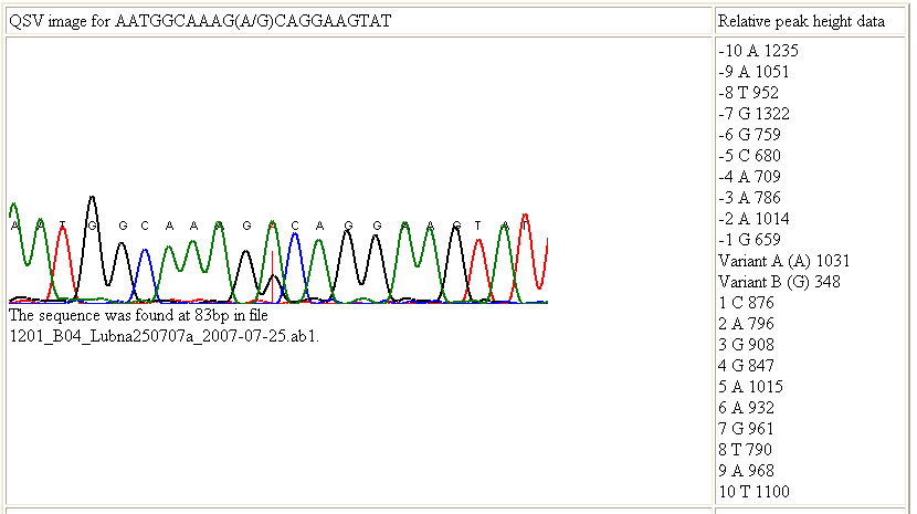
Figure 9: The first section of the web page contains details of the relative peak heights of the residues in the region of interest.
The second section shows batch statistics, namely the mean and standard deviation of the relative peak heights for each nucleotide, among all the files analysed (Figure 10). This information should be used to ensure that the nucleotides selected as reference peaks do not vary excessively compared to other nearby positions and that the intra-batch variation is not unduly high. These issues can be conveniently judged from the final column of the table in this section (standard deviation as a fraction of peak height).
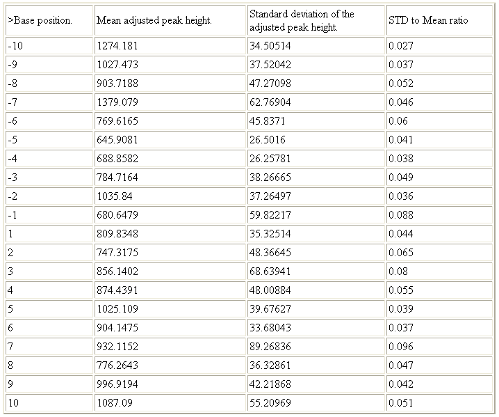
Figure 10: Mean values and the standard deviation for each nucleotide’s adjusted peak heights are shown in the second section of the web page output.
The final section shows the relative corrected peak height for each variant and the peak height ratio for each trace file. This value is given rounded to one and three decimal places (Figure 11, green and red boxes respectively). This section also shows the peak height ratio uncorrected for the background levels of each variant (Figure 11, blue box).
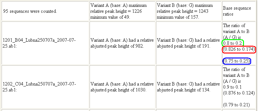
Figure 11: In the third section of the web page, the relative adjusted peak ratio for each trace file is shown, rounded to one and three decimal places (green and red boxes respectively), as well as the peak height ratio uncorrected for the background levels of each variant (blue box).
3 Practical considerations
3.1 Interpretation of results
While in most circumstances the true (chemical) copy number ratio can be directly approximated by the adjusted peak height ratio, this should always be verified, by the inclusion of sequence traces derived from samples with known copy number ratios. For analysis of LoH or of germline mosaicism, using changes in a heterozygous SNPs peak height ratio, such standards could be constitutional DNA from non-mosaic heterozygous individuals. Sequences representing paralogous duplicated targets must be calibrated against samples of known copy number, identified by other means such as Array CGH or Affymetrix SNP chip data. In most situations, these samples can be obtained from cell lines whose copy number has been published or is shown in public databases such as the UCSC Genome Browser (1), which contains copy number information from (2).
3.2 Inclusion of controls
To calculate the QSV ratio, the program needs two reference sequences, each containing only one of the two variants. Since the analysis depends on these sequences, and since it is unadvisable to cross-compare sequence data from a different sequencing runs (due to batch effects), it is recommended to include duplicates (or triplicates) of these reference samples in each batch.
3.3 Selection of sequence variant
If a number of possible QSVs are available to test for a particular purpose, we recommend using a variant where the two neighbouring nucleotides are both different to each of the QSV variant bases. The effect of a neighbouring residue that matches one of the QSV variants depends on the sequence quality. For example, if the individual nucleotide peaks have started to spread, then the flanking and variant peaks may merge into each other, and so the peak height of the variant is affected by the flanking base (Figure 12).
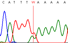
Figure 12: Individual peak of the same base type may merge into each other and variably elevate the peak height of the QSV nucleotide.
It is also important to check the effect of forward and reverse sequencing, since certain sequences suffer less from dideoxynucleotide incorporation bias in one direction than the other (Figure 13).
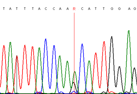
A
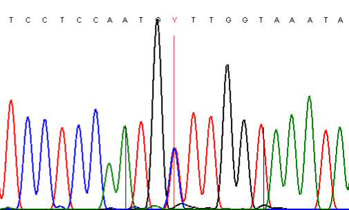
B
Figure 13: Dideoxynucleotide incorporation bias differs, according to the direction in which a PCR product is sequenced; A and B show the trace data for the same PCR product sequenced in the forward and reverse directions, respectively.
3.4 Computer requirements
We have run this program on both Windows Vista and Windows XP SP2. The computer must have the Microsoft .NET Framework Version 2.0 installed, which can be obtained through Windows Update or downloaded as a package from here.
4 References
(1) Kent WJ, Sugnet CW, Furey TS, Roskin KM, Pringle TH, Zahler, AM, Haussler D (2002) The Human Genome Browser at UCSC. Genome Res 12: 996-1006.
(2) Bailey JA, Yavor AM, Massa HF, Trask BJ, Eichler EE (2001) Segmental duplications: organization and impact within the current human genome project assembly. Genome Res 11: 1005-17.