User guide
Introduction
AgileVariantViewer allows sequence variants identified by AgileAnnotator (and optionally pre-filtered by AgileKnownSNPFilter) to be interactively filtered in order to facilitate identification of genuine (and possibly pathogenic) mutations. The filtering process can be performed by adjusting the cut-off parameters for read depth and the minor allele frequency. Variants can also be selected based on their position within a gene (exon, intron, splice site or Kozak start site). It is also possible to select variants by type (point mutation or indel) and by predicted functional severity.
If the sequence variants have been pre-filtered by AgileKnownSNPFilter, variants may also be selected according to whether they have an RS number, have been identified by the 1000 Genomes Project, or have not been described before. By adjusting the read depth and the minor allele frequency parameters and observing the effect of this on known genuine sequence variants with RS numbers, it is possible to assess how the chosen cut-off values affect the detection of true variants.
Once the desired cut-off values have been settled upon, the resulting set of sequence variants, from a specific region, from a single chromosome, or from the entire genome, can then be exported. It is also possible to export only homozygous variants or heterozygous variants.
Data used in this guide
The download page contains a link to the PXDN sequence variant data used for the examples in this guide. This dataset was used to identify a PXDN mutation in consanguineous patients with a rare congenital eye defect (citation). The data is derived from an Agilent capture reagent that was used to select regions for which the patient was autozygous. However, the reagent also enriched for other regions for which the patient was not autozygous. Although the actual disease-causing variant is located on the tip of Chromosome 2p, this guide will concentrate on a larger autozygous region on Chromosome 20 (Figures 11 to 23) and on a heterozygous region on Chromosome 1 (Figures 1 to 6). Figure 14 does show the region containing the deleterious variant on Chromosome 2. The variants have been pre-filtered by AgileKnownSNPFilter.ATOH7 sequence analysis walk-through
While this document describes in detail the use of AgileVariantViewer with data used to identify the PXDN mutation, a second guide that demonstrates the identification of a mutation in ATOH7 can be found here. Unlike the PXDN example, to identify the disease-causing ATOH7 mutation, it proved necessary to screen the sequence variants found in this second data set using AgileGeneFilter.
File formats
A description of the file formats for the variant and read depth files used by AgileVariantViewer can be found here.
Entering data files
AgileVariantViewer requires three files: the genomic annotation file, the sequence variants file, and the read depth file, each of which is produced by AgileAnnotator. Genomic annotation files contain the sequences and positional information of the coding exons, as described by the Consensus CDS (CCDS) project, and are used in the detection and annotation of sequence variants by AgileAnnotator. It is VERY important that the genomic annotation files used to create and then view sequence variants refer to the same version of the CCDS and genomic reference data.
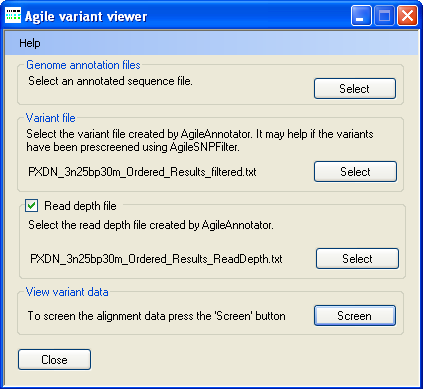
Figure 1: Selecting the data files
To select a genomic annotation file, press in the Genomic annotation file panel (Figure 1) and select the correct file. Since the file is large it may take a few moments to read. Next press in the Variant file panel (Figure 1) and select the file containing the sequence variants identified by AgileAnnotator. Finally, if you have a read depth file press in the Read depth file panel (Figure 1) and select the file containing the read depth data calculated by AgileAnnotator. If you do not have a read depth file, e.g. the variant data file was created by AgileFileConverter, uncheck the tick box in the Read depth file panel. Once all the files have been selected, press in the View variant data panel to display a graphical view of the data (Figure 2).
Viewing the sequence variant data
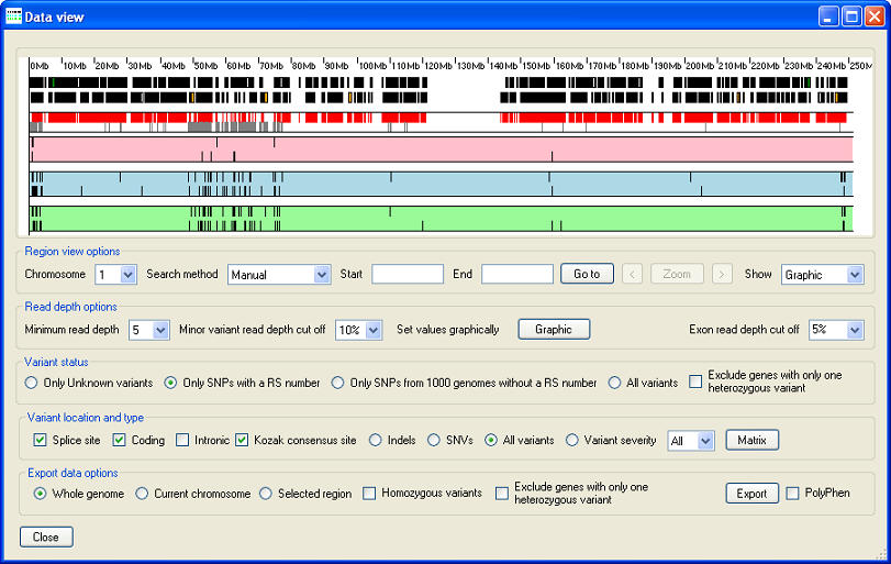
Figure 2: The Data view window displays the variant data.
When the Data view window opens, it displays a graphical view of the sequence variant data on Chromosome 1 in its upper panel (Figure 2). However, an alternative view, of the exon read depth as a histogram, can be selected (Region view options → → “Read depth”). This option is described in greater detail below under Viewing the exonic read depth data (see Figure 15). Below the graphical display panel are five “options” panels which allow the sequence variants to be filtered and then exported. Each of these panels is described in detail below:
Description of the sequence variant display panel
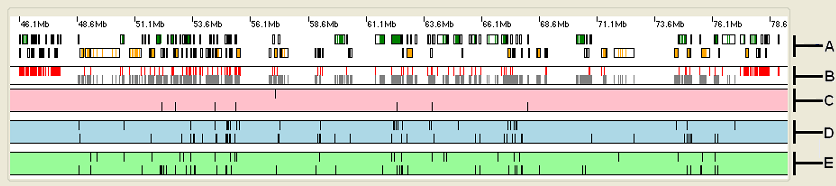
Figure 3: The upper panel displays the analysis data organised as a number of horizontal strips.
The upper panel displays the analysis data organised as five horizontal strips (Figure 3).
- Strip A: shows the location of any genes (black rectangles) in the selected region, with the green and orange rectangles representing exons transcribed from
the positive and negative DNA strands respectively.
Placing the cursor over any gene in this strip causes the gene’s name to appear in the window’s title bar. - Strip B: shows the positions of exons whose typical read depth is above (grey block) or below (red block) the cut-off value selected from the list in the Region view options panel (see below).
- Strip C: shows the locations of sequence variants that are likely to affect the function of a protein. These include those that create in-frame stop codons, frameshift variants (indels), splice site variants and those that disrupt the gene’s normal stop codon. The vertical lines in the upper part of the strip represent homozygous variants, while those in the lower part of the strip correspond to heterozygous variants.
- Strip D: shows variants that alter the amino acid sequence of a protein, as well as those close to the start codon which might affect protein translation. These variants have a intermediate (and indeterminate) risk of altering the protein’s function. The vertical lines in the upper part of the strip represent homozygous variants, while those in the lower part of the strip correspond to heterozygous variants.
- Strip E: shows sequence variants that are less likely to affect a protein’s function, since they are either in an intron or do not alter the amino acid sequence. Again, the vertical lines in the upper part of the strip represent homozygous variants, while those in the lower part of the strip correspond to heterozygous variants.
Selecting a genomic region to view
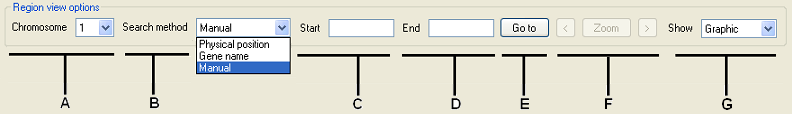
Figure 4: Selecting genomic regions to view is performed using the Region view options panel.
The Region view options panel contains the controls that allow different genomic regions to be viewed (Figure 4). The list (Figure 4, labelled A) is used to select the chromosome to view. A chromosomal region may be selected by entering the region’s coordinates, by entering the gene names of the genes flanking the region, or by mouse-clicking on the graphical view in the upper panel.
- To select a region by entering its coordinates, select the “Physical position” option in the list (Figure 4, labelled B) and enter the basepair coordinates of the region in the and boxes (Figure 4, labelled C and D). Next, press the button; this should place two vertical black lines on the graphical data view, identifying the selected region. Finally, if the selected region is correct, press the button to view the region.
- To select a region using names of the flanking genes, select “Gene name” from the list and enter the names of the genes at the region’s start and end points in the and boxes (Figure 4 C and D). (To view a single gene, enter the same name in both text boxes). Next, press (Figure 4, labelled E); this should place two vertical black lines on the graphical data view, identifying the selected region. Finally, if the selected region is correct, press (Figure 4, labelled F) to view the region.
- To select a region by mouse-clicking on the graphical view panel, select “Manual” under (Figure 4, labelled B), right mouse-click on the graphical view panel at the end of the region, and then left mouse-click at the start of the region. Finally, if the selected region is correct, press the button (Figure 4, labelled F) to view the region.
Pressing the and buttons (Figure 4 F) moves the selected region to the left or right of its current position by 90% of its width, so that 10% of the previous view is retained.
The Region view options panel also contains the options list (Figure 4, labelled G). If the “Graphic” option is selected from this list, the sequence variants graphical view shown above is displayed. Alternatively, the “Read depth” option will invoke a histogram display of the exonic read depths. See Viewing the exonic read depth data and Figure 15.
Adjusting the sequence variant filtering parameters
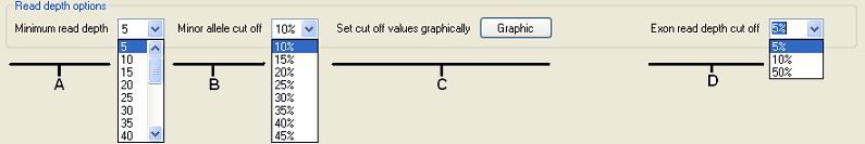
Figure 5: The Read depth options panel interactively filters the sequence variants by read depth and minor allele frequency.
The Read depth options panel allows the sequence variants to be filtered by adjusting the minimum read depth and minor allele cut-off parameters, which are used to genotype a sequence variant. When either of these parameters is altered, the graphical display in the upper panel is updated, allowing the effect of each change to be seen. To adjust the minimum read depth at which a sequence variant is called, select a new value from the list (Figure 5, A), while to change the minor allele frequency cut-off value, select the appropriate value from the list (Figure 5, B). Changing either of these values causes the graphical panel to update both the view of sequence variants that pass the selected parameters and the list of exons whose read depth is above the new minimum read depth. Whether an exon passes the minimum read depth depends on the minimum read depth parameter used to screen the sequence variants and on the exon read depth cut-off. This parameter can be set to 5%, 10% or 50% using the list (Figure 5, labelled D). If set to 5%, then for an exon to pass, 95% of all its protein-coding positions must be covered by a read depth equal to or greater than the minimum read depth value used to filter the sequence variants. (Similarly, if the value is set to 10% or 50% then, 90% or 50% of the protein coding positions in an exon must have a read depth equal or greater than the minimum read depth parameter.) Exons which fail this test are drawn as red rectangles in the strip labelled B in Figure 3, while those that pass the cut-off are drawn in grey.
The effect of adjusting the sequence variant cut-off parameters
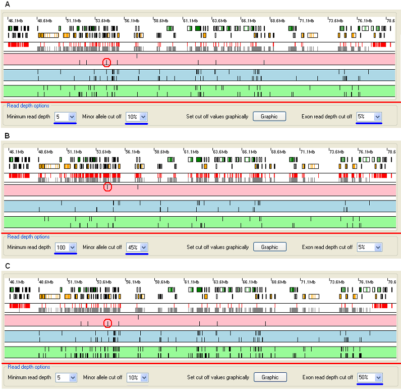
Figure 6: The effect of adjusting the sequence variant cut-off parameters.
Figure 6A shows the graphical display of a heterozygous (non-autozygous) region, viewed with the default cut-off settings (note values underlined by the blue lines). If the cut-off parameters are now increased (Figure 6B, adjusted values underlined by blue lines) the proportion of sequence variants and exons that fall below the new cut-offs increases. This is seen as an increase in the number of red rectangles in the exon read depth strip (Figure 3, A) and a decrease in the number of vertical lines in the pink, blue and green sequence variant strips (Figure 3 B, C, D).
Spurious heterozygous sequence variants may arise due to basecalling errors at positions that are actually homozygous either for the reference allele or a variant allele. As the minor allele frequency cut-off is increased, heterozygous sequence variants will progressively decrease in number and will convert to homozygous, either for the reference sequence or for a variant allele. Homozygous wildtype positions are not displayed, but homozygous variant positions are. Therefore as the value is increased, the number of heterozygous variants decreases, while the number of homozygous variants may increase. The red circles in Figure 6 highlight a variant that changes from heterozygous to homozygous as the cut-off values change.
The effect of changing the from 5% (Figure 6A) to 50% can be seen in Figure 6C. Since only 50% (rather than 95% in Figure 6A) of the protein-coding positions in an exon must now be above the cut-off for a exon to pass, there are fewer red rectangles in the exon read depth strip (Figure 3, A) than in Figure 6A and 6B.
Adjusting the read depth and allele frequency cut-offs using the “Variant reads depths” window
In addition to the above, it is possible to interactively modify the read depth and allele frequency parameters using a second graphical interface, the Variant reads depths window. In this, sequence variants are plotted according to the read depths of their reference and variant alleles (Figures 7 to 10). The window is displayed by pressing the → button (Figure 5, labelled C).
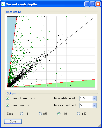
Figure 7: The Variant reads depths window displays a graph of the reference allele’s read depth (Y-axis) against the variant allele’s read depth, for each single nucleotide sequence variant. Grid lines are drawn at read depth intervals of 100.
The reference allele’s read depth (Y-axis) is plotted against the variant allele’s read depth, for each single nucleotide sequence variant. Differently coloured regions identify the sequence variants which are homozygous for the variant allele (green), heterozygous (white) and homozygous for the reference allele (pink). The blue region corresponds to positions at which the minor allele read depth was below 10% and so the position was not called. The smaller red triangle close to the origin of the graph shows the region where the read depth is too low to call a position. If the sequence variants were previously filtered by AgileKnownSNPFilter, each variant is drawn as a green dot (unknown variant) or a black dot (present in the 1000 Genomes data set). (If not previously filtered, all the variants will be drawn as green dots.) The black diagonal from bottom left to top right shows the line around which heterozygous sequence variants should fall.
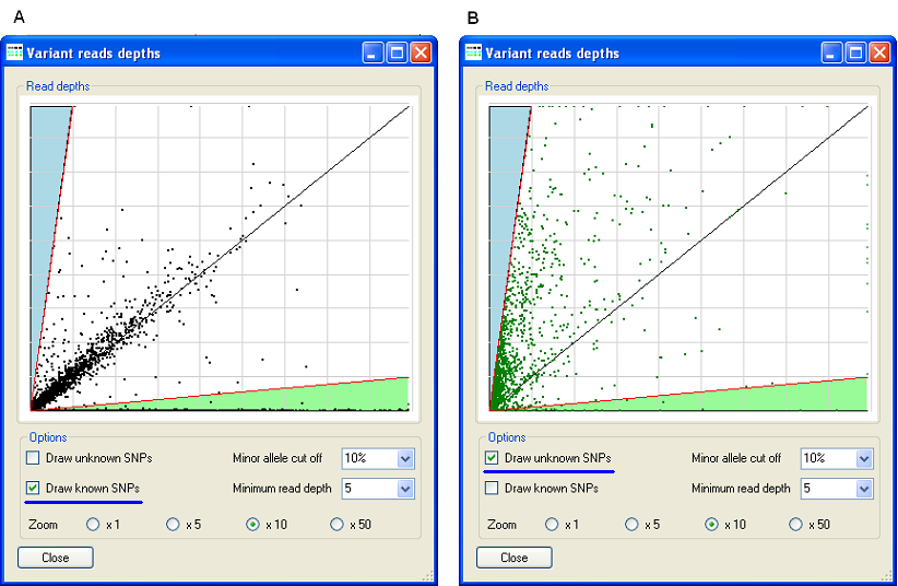
Figure 8: Displaying only already known (Figure 8A) or unknown (Figure 8B) sequence variants.
It is possible to display only known (Figure 8A) or only unknown (Figure 8B) sequence variants by ticking the corresponding box in the Options panel. When only known SNPs are displayed (Figure 8A), it can be seen that most of the variants lie either close to the X-axis (homozygous for a variant allele) or along the black diagonal (heterozygous). In contrast, when only unknown SNPs are displayed, it may be noted that the distribution is less well defined, with a large proportion of apparent variants lying closer to the Y-axis. This suggests that most of these novel variants are actually false positives.
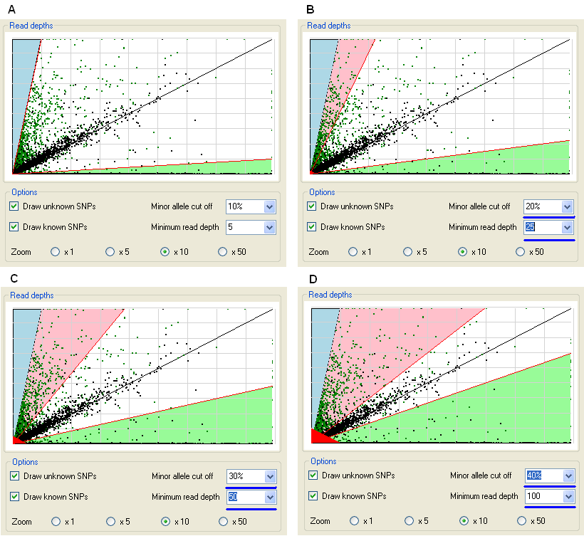
Figure 9: the graph is updated when the read depth and minor allele frequency cut-off values are altered.
The read depth and allele frequency ratio cut-off values can be interactively adjusted using the and boxes on the Options panel. When these parameters are changed, the graphics both in this window and the Data view window are updated. Figure 9 shows the effect of changing these values on the extent of the coloured regions of the graph. As the minor allele frequency value is increased, the areas of the pink and blue sectors (encompassing homozygous variants) increases, while the white, heterozygous region shrinks. Similarly, as the minimum read depth cut-off increases, the size of the red triangle in the bottom left corner of the graph increases. Since most known SNP variants are probably true positives, it is better to use such known variants as a guide for adjusting the minor allele frequency, so that the white region is as small as possible, while still including most of the variants close to the diagonal line.
Viewing an autozygous region
In the figures above, a heterozygous region is shown; for such a region, it is often not possible to know whether a detected variant is a true or a false positive. In contrast, the remaining figures below relate to an autozygous region, within which it is reasonable to believe that all heterozygous variants represent false positives.
Viewing different classes of filtered SNPs
If the sequence variants have been filtered by AgileKnownSNPFilter choices are available to view sequence variants that have a RS number, sequence variants that are in the 1000 Genomes Project data set but have no RS number, previously unknown sequence variants, or all sequence variants. Figure 10 demonstrates the effect of viewing each of these classes of sequence variant, across an autozygous region (on Chromosome 20, in the PXDN data set). Since this region is autozygous, all apparently heterozygous variants are false positives.
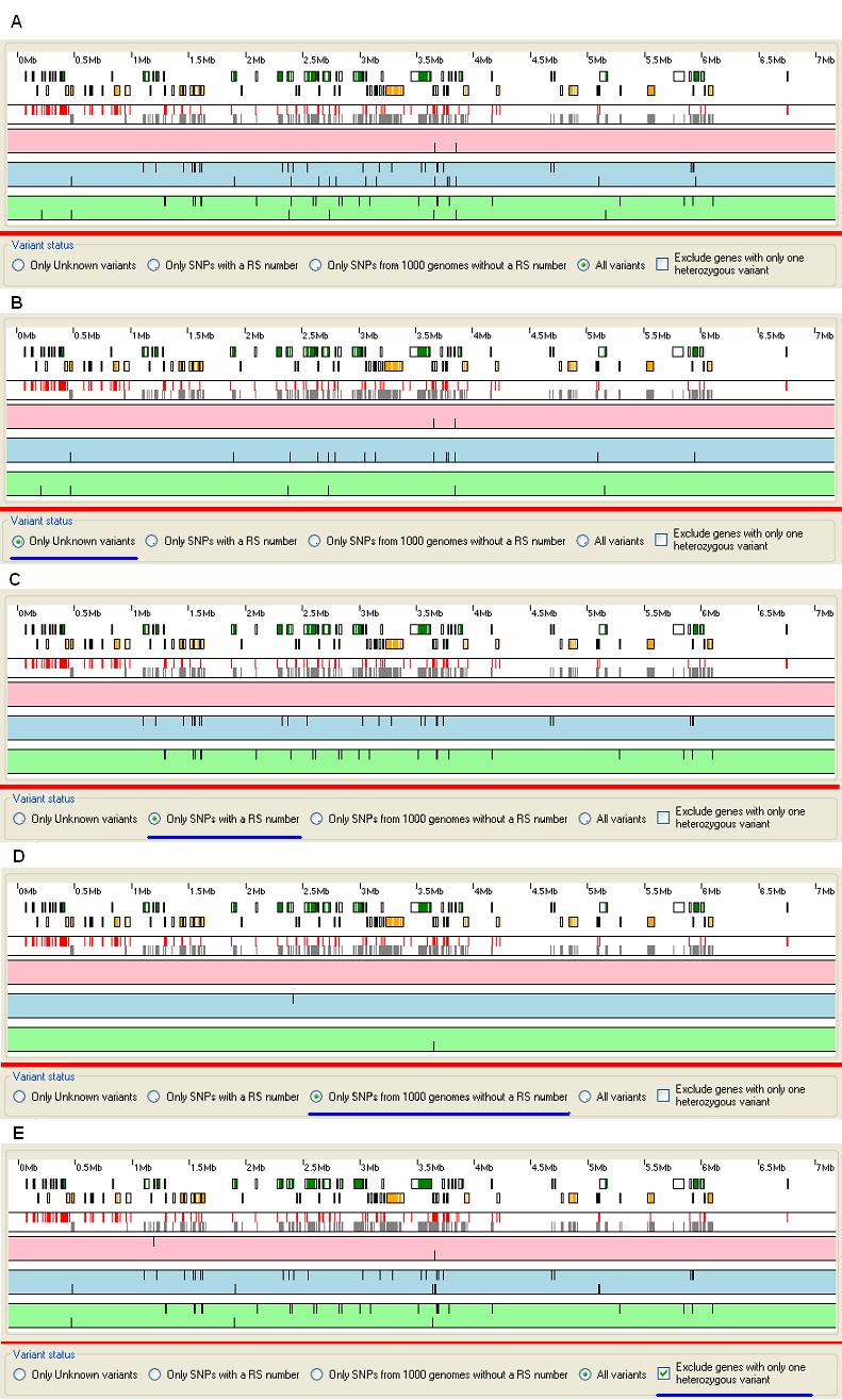
Figure 10: Displaying different classes of sequence variants.
The , , and options on the SNP status panel allow each class of filtered sequence variant to be displayed (Figure 10). When all sequence variants are displayed (default setting), both homozygous and heterozygous sequence variants appear to be present (Figure 10A). However, since this region is autozygous, it can be assumed that the heterozygous variants are actually false positives. Furthermore, when only unknown sequence variants are selected for display (Figure 10B), it can be seen that only heterozygous SNPs remain shown, suggesting that most of these variants are again false positives. Conversely, when only sequence variants with an RS number are displayed (Figure 10C) only homozygous variants are now visible, suggesting that most of these variants are true positives. Finally, selecting variants that have been seen in the 1000 Genomes Project but do not have an RS number leaves only two variants, one of which is probably a false positive. This result is interesting, given that 55% (296,456 / 538,332) of the sequence variants used by AgileKnownSNPFilter to filter the sequence variants fall into this category.
Viewing sequence variants by location relative to genomic features
The location of a sequence variant within a functional feature of a gene (exon, intron, splice site or Kozak consensus site) can be a strong predictor of the variant’s severity. Therefore, the program can display the set of variants identified in each of these locations.
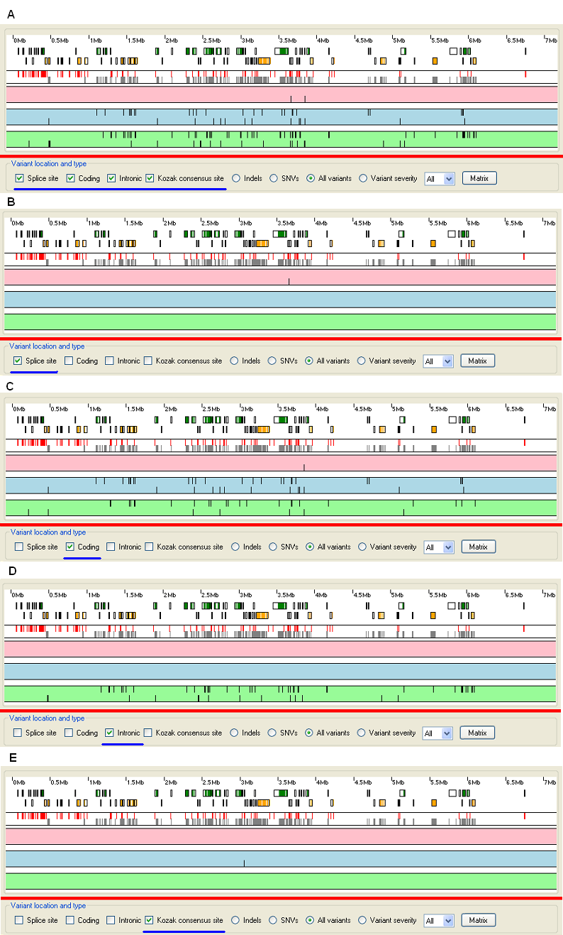
Figure 11: Displaying sequence variants according to location within different parts of a gene
The , , and options on the Variant location and type panel allow sequence variants to be displayed depending on their location within one of these elements (Figure 11). By default, variants in the exons, splice sites and Kozak consensus sequence are displayed. However, it is possible to display sequence variants located within any combination of gene features. For example, Figure 11A shows variants from any of the features, whereas in 11B to 11E those from each of the categories in turn are shown.
Since variants within splice site consensus sequences probably affect mRNA splicing, they are always displayed in the pink strip of the display. Conversely, intronic variants outside splice sites are more likely to be benign, and so are always placed in the lower green strip. Since the effect of a Kozak site variant cannot easily be predicted, these are displayed in the blue strip. Exonic variants may be placed in any of the three strips, with silent changes placed in the green strip. Those that disrupt the protein sequence (frame shifts and those that create or destroy stop codons) are placed in the upper pink strip, with the remaining (missense) variants displayed in the blue strip.
Displaying sequence variants based on their possible severity
Since sequence variants that alter or disrupt a protein sequence are the most likely to be pathogenic, the displayed variants can be filtered according to simple categories that may influence severity of impact (Figure 12).
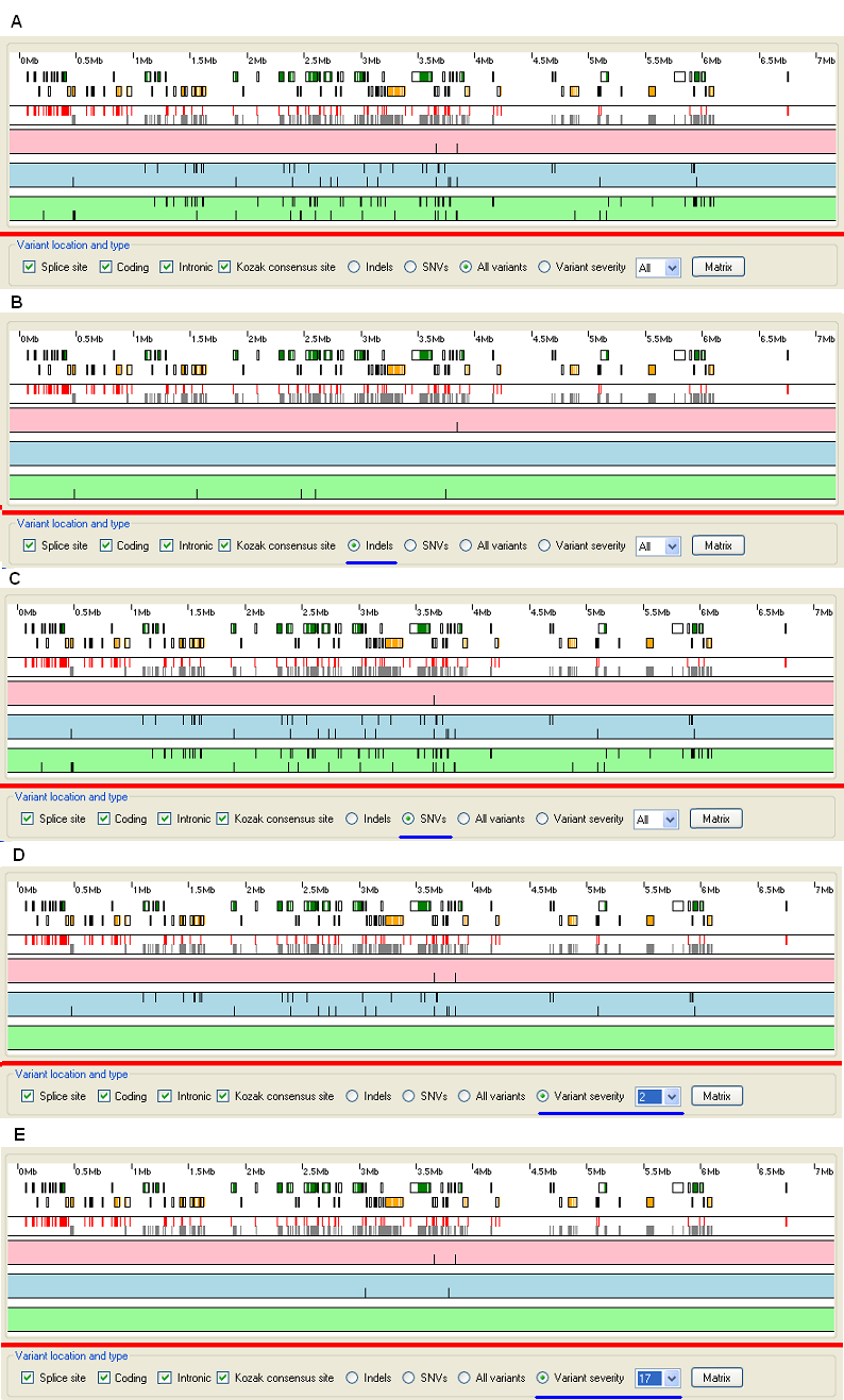
Figure 12: Displaying sequence variants based on their possible severity.
While it is possible to display all the sequence variants identified in a region (Figure 12A) it is also possible to select variants based on their possible severity using the , , and options on the Variant location and type panel. By default, the option is selected (Figure 12A). If the option is selected, only insertions or deletions are shown (Figure 12B), with intronic indels always appearing in the lower green strip and exonic and splice site indels appearing in the upper red strip, since they are very likely to disrupt protein structure and function. Given that the region shown in Figure 12 is autozygous, so that all heterozygous variants are likely to be false positives, it is noteworthy that all the indels in the region are heterozygous and so probably not genuine. Selection of the options displays the single base change variants, which since they vastly outnumber the other variant classes, creates a display very similar to the default option.
When using the option, the severity of each sequence variant is calculated using a matrix derived from the scoring system used by the BLASTP alignment algorithm to align protein sequences. The matrix scores how likely it is, during evolution, that one amino acid will be substituted, and how often a particular substitution occurs. A conservative change like alanine to glycine scores 1, whereas a tryptophan to cysteine change scores 25. This scoring system is simplistic and does not take into account any structural information. For example, glutamate to aspartate scores 4, suggesting a modest effect, but if an individual glutamate is used to bind a zinc atom, this substitution might nonetheless disrupt an enzymatic activity. Despite these restrictions, since the BLASTP scoring system is easily performed, it can be useful for quick screening of variants during a preliminary analysis. The cut-off value for this function is set using the options list to the right of the option. Pressing the button allows the scoring matrix to be saved to disk as a web page. Selecting the option and setting the cut-off value to 2 causes the variants in the green strip to be hidden, along with a small number of variants in the blue strip (Figure 12D). However, setting the cut-off value to 17 causes the majority of sequence variants to be discarded; furthermore, those that remain are all heterozygous, suggesting that they are false positives (Figure 12E).
Exporting filtered sequence variant data
It is possible to export the sequence variants, using the same criteria as that used to display them in the graphical display, by using the setting in the Export data options (Figure 13). For instance to export sequence variants that have not been found by the 1000 Genome project and do not occur in intronic sequence, select the option in the SNP status panel (Figure 10) and select the , , and options on the Variant location and type panel.

Figure 13: Exporting filtered sequence variant data.
Once the various parameters have been set, it is possible to export the sequence variants that meet these cut off values by pressing the button in the Export data options panel (Figure 13). If there is no positional information available, it is possible to export sequence variants from the whole genome by selecting the option in the Export data options panel (Figure 13). Otherwise it is possible to export sequence variants from either the currently selected chromosome or chromosomal region, by selecting the appropriate or option in the Export data options panel (Figure 13). If the disease causing variant is believed to be homozygous, it is possible to export only homozygous variants by ticking the boxes. Similarly, if the patient is believed to be a compound heterozygote, ticking the will export heterozygous variants only if two or more heterozygous variants are present in the gene. Selecting both of the options will export both sets of variants. If the condition is believed to be dominantly inherited then do not select either of these options.
Considerations when setting the selecting parameters
The majority of unknown sequence variants appear to be false positives, while the majority of sequence variants with a RS number appear to be true positives. Similarly a severe sequence variant is more likely to be a false positive than a benign sequence variant. Therefore, the cut off parameters should be set so that they discard as many unknown variants as possible while keeping as many variants with a RS number. Similarly, the parameters should discard as many severe variants as possible while lossing as few benign variants as possible. When the cut off parameters have been set, only export unknown variants.
This guide shows data for two regions from a single sequencing run on a DNA sample selectively enriched for specific regions. Neither of these regions contained the disease causing variants, however the mutation is present in the PXDN data file and is located in a small autozygous region at the start of chromosome 2 (Figure 14). Figure 14A shows the display with the default cut off parameters, while Figure 14B show the display after the parameters have been adjusted to display unknown, coding variants tha affect the proteins's amino acid sequence. Initially, the variant was identified as heterozygous due to the presence of a small proportion of erroneous base reads at this position.
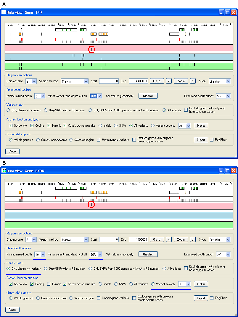
Figure 14: The disease causing mutation in the PXDN data file is located at the start of chromosome 2 in the PXDN gene and highlighted by the red circle, before (Figure 14A) and after (Figure 14B) the parameters where adjusted.
Viewing the exonic read depth data
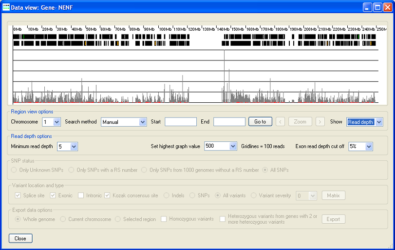
Figure 15: When the 'Read depth' option from the list in the Region view option panel is selected the exon read depth data is displayed as an histogram. (The data displayed in Figure 15 is derived from an exome sequence analysis.)
By selecting the 'Read depth' option from the list in the Region view option panel (Figure 14) the read depth data for each exon is shown as a histogram. As well as changing the graphical display, selecting this option removes the list and the button from the Read depth options panel, replaying them with the option. Also selecting this option dispbles the SNP status, Variant location and type and Export data options panels. As before it is possible to select different genomic regions using the options in the region view options.
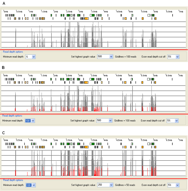
Figure 16: Modifying the exon read depth histogram. (The data displayed in Figure 15 is derived from PXDN pulldown sequence analysis and shows the same region as Figures 10 to 13.)
When the exonic read depth for an exon is above the minimum read depth value selected in the list, in the Read depth options panel, it is drawn as a grey rectangle, otherwise it is draw in red. The affect of changing this value can be seen by comparing Figure 16A (minimum read depth = 5) to Figure 16B (minimum read depth = 100). The maximum read depth value shown by the graph is set using the list in the Read depth options panel. The affect of changing this value from 500 to 250 is shown between Figures 16B and 16C. The text to the right of the list shows the read depth interval of the horizontal lines in the graph.