A program for collecting peak signal intensity levels from ABI genotype files
Application to detection of germline microsatellite instability in patients suspected of suffering from MMR-D
Overview
This program is designed to automate the process of collecting PCR product peak signal intensity levels from ABI genotype files (*.fsa). There is no pre-set minimum hardware specification, but the computer must run the Microsoft .NET Framework 2.0. The length of time needed to analyse each data set will depend on the size and number of files in the analysis.
Getting started
Since PeakHeights is designed to process several files per run, data entry is performed by selecting a folder containing all the *.fsa files to be analysed. To select the desired folder, choose the option from the menu (Figure 1a), browse to the folder using the displayed form, and then press . (Files with other filename extensions will be ignored.)
Once the input files have been read, the trace information is displayed in the form of a “virtual gel”, with lanes as vertical strips (10 pixels wide) in the central panel of the display window. These strips display only the red channel signals and are oriented with the first scan at the top of the panel (Figure 1b). The vertical scale and starting point for the displayed image can be adjusted using the text boxes in the bottom left of the form. Similarly, the intensity of the image can be altered using the Maximum intensity text box. Any signal intensity greater than this value is shown as black, while lower values are scaled linearly between white (intensity = 0) and black (intensity = value). After adjusting any of these values, press to update the image. Should the combined width of the traces exceed the panel width, the horizontal scroll bar below the panel can be used to navigate along the image.
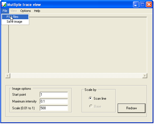
Figure 1a
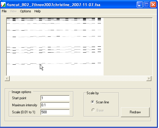
Figure 1b
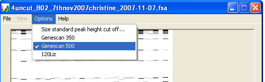
Figure 1c
Calibrating the traces to the size standard
By default, PeakHeights uses the ABI Genescan 500 size marker to calculate the sizes of the experimental products. Alternatively, the Genescan 350 marker set can be selected using the menu (Figure 1c).
Since the absolute migration rate of a PCR product varies between capillaries, each trace must be calibrated against the size standard. To do this, left-click on the desired trace in the main panel. This brings up a graph showing scan number (x axis) and signal intensity (y axis; maximum = 1500) for all four dyes (Figure 2a). Since this image is not scaled to fit the panel area, absolute signal intensities can be judged.
Peaks are defined as regions of signal intensity that are greater than the cut-off threshold and flanked by regions of <85% of the threshold. These values are shown by the horizontal black lines across the graph. When two peaks merge at their bases, both black threshold lines should be positioned to lie between the peaks’ maxima and the point at which they merge. Similarly, when peaks are faint, the threshold should be reduced to a suitable value less then the peak intensity. To change the cut-off value, select and enter a new threshold value (Figure 2b). The program will then calculate the lower 85% value and re-analyse the files.
[Note that despite this threshold filter, when the time comes for data export (see below), it will be possible to explicitly specify PCR product sizes for export, irrespective of whether their intensities meet the specified threshold, or whether the program identifies them as peaks.]
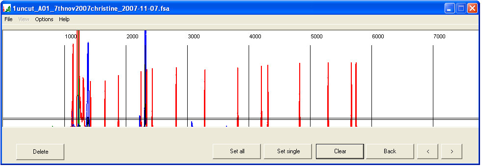
Figure 2a
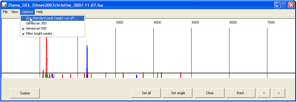
Figure 2b
Setting the marker sizes
Generally, it is only necessary to manually assign sizes to two marker peaks (which must define the upper and lower limits of the region of interest). To assign a marker size, left-click over its peak. The program will look for the peak nearest to the cursor, prompt the user to enter a size in base pairs, and assign that size to the peak (Figure 3a–b). Where two peaks are close together (e.g. 340 bp and 350 bp markers) care must be taken that the correct peak has been selected. The program will automatically calculate the remaining peak sizes (Figure 3c).
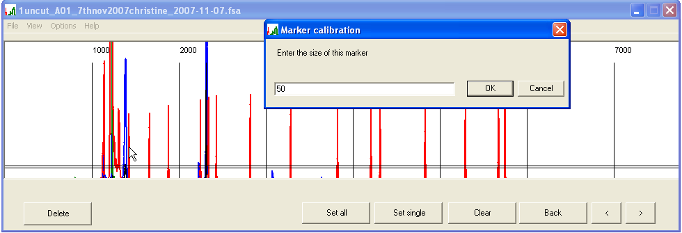
Figure 3a
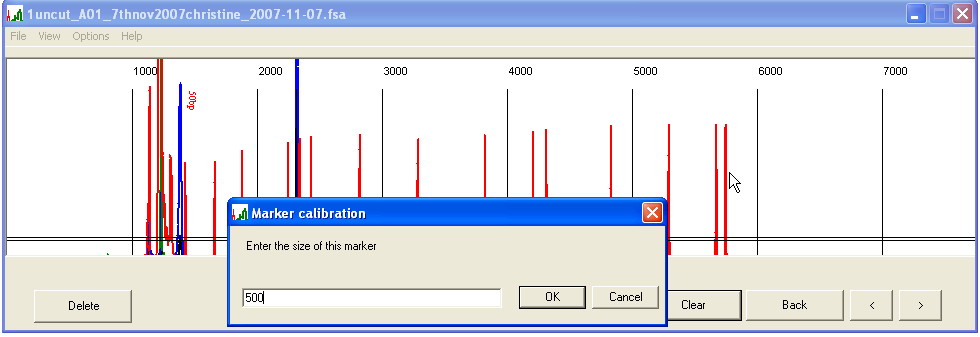
Figure 3b
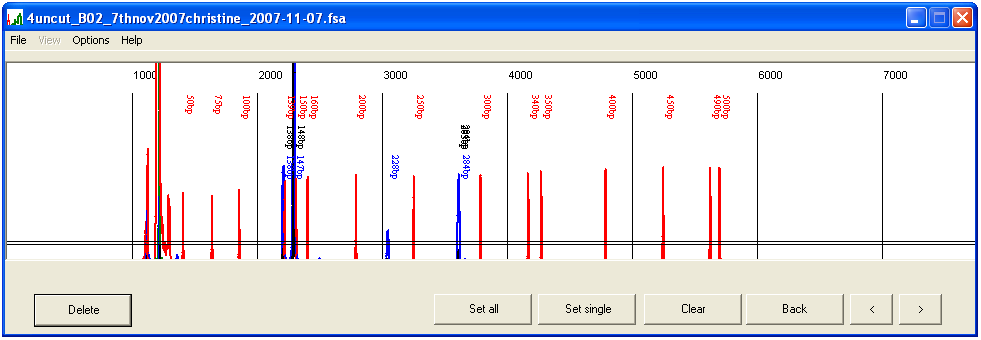
Figure 3c
Assigning the first and last marker sizes as above suffices for most situations. However, migration rates may be anomalous if the capillary is overloaded or the sample contains excessive contaminants. In such cases, first select the smallest marker peak and then an intermediate peak (~160 bp), before selecting the upper size range. If the program does not correctly score the marker sizes, pressing the button will remove the current size data, whereupon the procedure can be repeated, using a smaller interval between each manually assigned size marker.
If a trace is of low quality, it can be removed from the dataset using the button. Pressing the button will discard the calibration data and return to the original window.
Calibrating all the files in the dataset and check for miscalls
Once one trace file has been calibrated as described above, pressing the button uses this marker information to calibrate all the other files in the data set. Once this has been completed, the original form reappears. To see how well each trace has been calibrated, select the Scale by... Base radio button (Figure 4) and press . The panel will then show the signal intensity scaled to its base pair position, rather than scan number. (Compare Figures 1c and 4.)
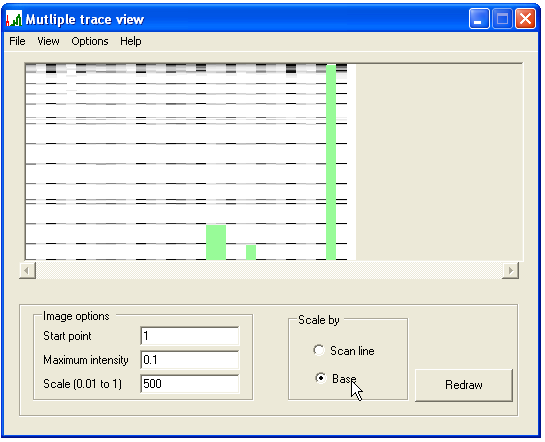
Figure 4
The program calibrates sizes working from smallest to largest marker. If it is unable to calibrate the end of a trace, the uncalibrated region is shaded green (Figure 4). If an internal region has been incorrectly calibrated, it will be noticeable as a region where the size markers do not align with those in the rest of the data set. To view the calibration of a single trace, left-click the trace in the main panel, view its graph in the calibration panel (as in Figure 3) and if necessary recalibrate the trace. This recalibration can then be saved without affecting the calibration of the other trace files, by pressing .
Viewing calibrated trace data
Once the trace data have been calibrated, the electropherograms can be viewed by selecting from the menu. The resulting Scan view window displays the first four electropherograms from the data set (Figure 5). Different trace files can be viewed by selecting their names from the drop-down list boxes above each electropherogram. To view a sub-region of the traces, drag with the left mouse button over an area of the display (Figure 6a): when the mouse button is released, the display will zoom to the selected region (Figure 6b). To revert to the original scale, simply left-click the image.
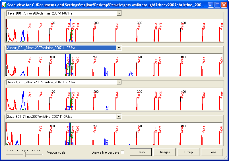
Figure 5
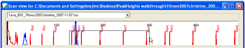
Figure 6a
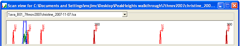
Figure 6b
Calculating gMSI ratios
Pressing the button on the Scan view window opens the Peak ratios window (Figure 7). The Data display panel displays the data for a single file and shows the same size interval as selected in the Scan view window. However, the vertical scale of the peaks is automatically adjusted so that the largest peak under analysis is 90% of the height of the display panel. The data file displayed is selected by choosing the appropriate filename from the file selection list. The individual fluorophore/trace colour displayed is selected using the appropriate colour option below the Display panel .
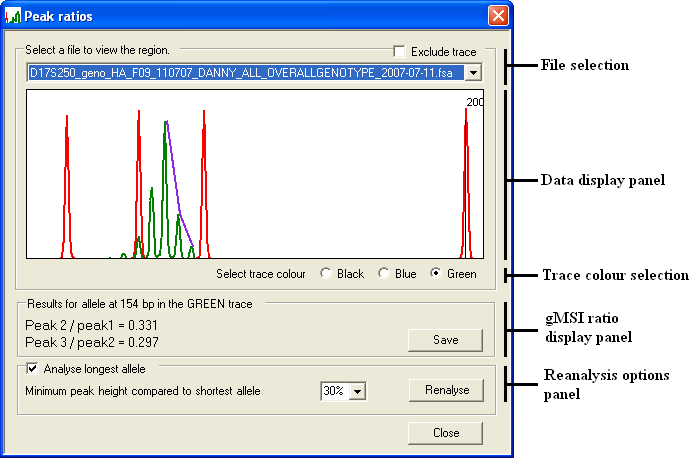
Figure 7
The gMSI ratio is determined by dividing the height of an allele’s trailing “stutter” peak by the height of the allele’s major peak. The peaks currently under analysis are identified by a purple line connecting the tip of each peak. The program also calculates the gMSI ratio for the next pair of stutter peaks. While this ratio is more variable than the ratio derived from the major and first stutter peaks, it can provide supporting evidence for a gMSI ratio, with both values generally being similar. If these two values are very different, then the original microsatellite may need to be re-amplified and the analysis repeated. The values of these two ratios are displayed in the gMSI ratio display panel. The legend text for this panel also displays the size in bp of the microsatellite allele being analysed.
By default, PeakHeights selects the tallest peak as the major allele to analyse. However, if the patient is heterozygous for a microsatellite marker with overlapping alleles, the “stutter” peaks of one may interfere with those of the other (Figure 8a). If the box (on the Reanalyse options panel) is selected and the button is pressed, the longest allele will be selected (Figure 8b). To stop erroneous peaks from being selected, the new peak must be greater than a user-defined percentage of the size of the originally selected peak. The default value for this parameter is set at 30%, but can be adjusted by selecting a different value from the drop down list in the Reanalyse options panel and pressing the button.
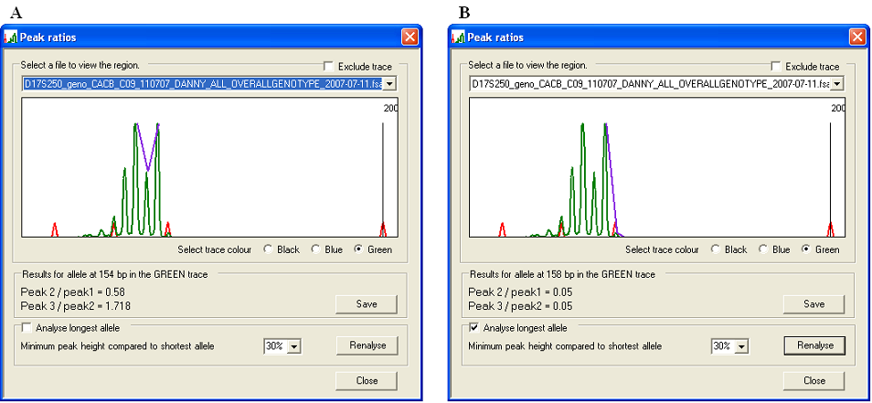
Figure 8
Exporting gMSI data
While viewing the each microsatellite file, it is possible to exclude a file from the final analysis by ticking the box located at the top of the Data display panel (Figure 7). This does not delete the file itself, but stops the marker’s gMSI ratio and peak height data from being exported. Pressing in the gMSI ratio display panel saves the gMSI ratio values and the analysed peak’s heights to a tab-delimited text file with a *.xls extension. This file can then be viewed and manipulated in a spreadsheet application such as Excel. An example of a data file created by PeakHeights is shown in Figure 9.
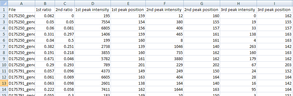
Figure 9
Example data
Example data from both normal and MMR-D patients can be downloaded from here: Normal individuals and Affected MMR-D patients
Exporting the signal intensity data
To export the desired peak intensity scores, from the Scan view window (Figure 5) press at the bottom right. This will open an Export data dialogue window (Figure 10). Before the data can be exported, the files of interest, PCR product sizes and dye colours must all be selected:
- Files to be exported: To add files one by one, select using the upper list box and press (Figure 10). To select all files, press . Selected files will be moved from the upper list box to the lower one. To deselect a file, highlight it in the lower list box and press . To deselect all files, use .
- The different dye channels can be selected or deselected for export using the three tick-boxes (Black, Blue, Green) (Figure 10).
- To discard information on peaks that are not of interest, either a size range or a set of specified peak sizes can be chosen, using the Sizes (Figure 11) and Range (Figure 13) tabs at bottom left. To specify individual peaks, enter a PCR product length in the Add this peak size box and press , repeating this procedure for each desired product size. To remove a size entry, select it from the Remove this peak size list box and press (Figure 11a). To avoid the need to repeat this manual selection, the chosen set of peaks can be saved for future use (and re-imported) using the File tab (Figure 12). To allow for the possibility that a peak size is miscalled by a single base, deselecting Analyse distinct peaks only (Figure 11b) will have the effect that two additional signal intensities (corresponding to the chosen product size +/-1bp) are also exported along with the selected peak’s intensity.
- To select all PCR product sizes that lie within a range, enter the upper and lower limits on the Range tab (Figure 13). Since it is simple to enter a size range, the option to save these values to a file is not available.
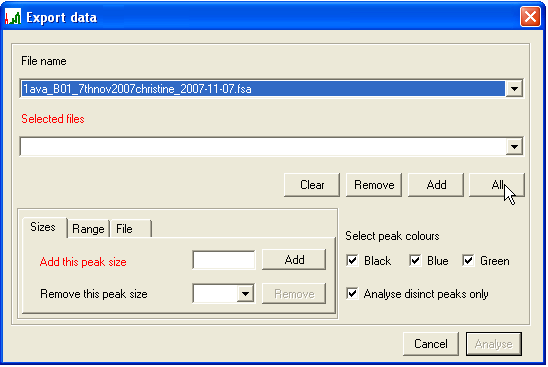
Figure 10
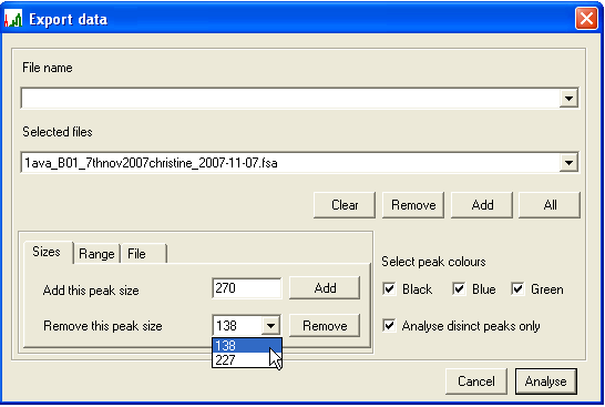
Figure 11a
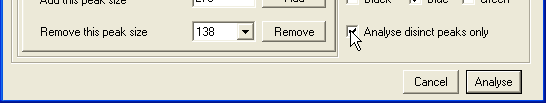
Figure 11b
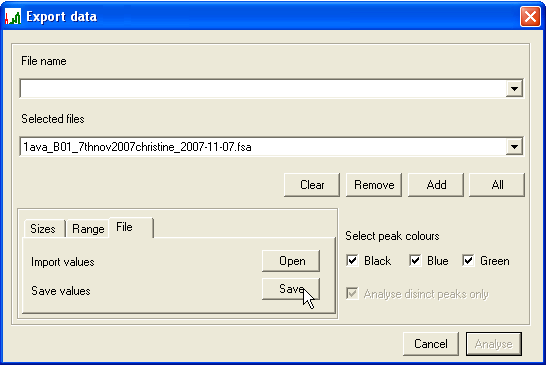
Figure 12
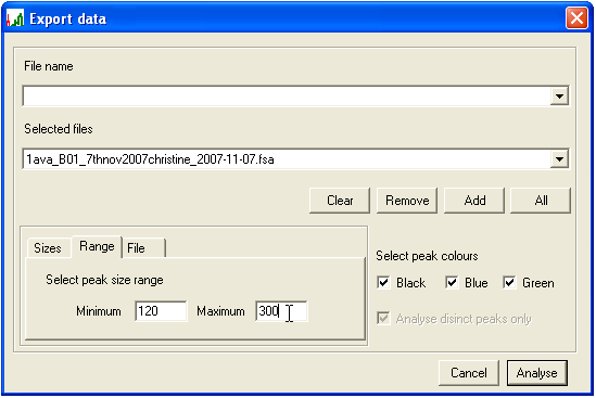
Figure 13
Once the required selections have been made, press . The Export data window will then close and the data will be saved to a tab-delimited text file with a *.xls file extension. If the Range function has been used to specify the exported peaks, only those peaks with intensities greater than the cut-off value specified during the size standard calibration will be exported. Products whose sizes were specified individually via the Sizes tab are not subject to this constraint, and their signal intensities are returned even if below the cut-off value.