User Guide
Overview
This program is based upon CpGviewer, which was modified for use in MAPit experiments as described in:
Jessen WJ, Hoose SA, Kilgore JA, Kladde MP (2006) Active PHO5 chromatin encompasses variable numbers of nucleosomes at individual promoters Nat Struct Mol Biol 13:256-63.
In common with CpGviewer, MethylViewer can analyse files from the ABI series of sequencers, as well as standard chromatogram format (*.scf) and plain text files. There is no preset minimum hardware specification, but the computer must run the Microsoft .NET Framework 2.0. The length of time needed to analyse each data set will depend on the number of files and the size of the reference DNA sequence. However, CpGviewer and MethylViewer differ in a few important ways (Table 1).
| Feature | CpGviewer | MethylViewer |
|---|---|---|
| Methylation sites | CG | Up to four user-defined sites per analysis |
| Bisulphite-treated strands | Clones of both sister strands in one analysis | Clones of only one sister stand |
| Web page view | Creates web page view | Does not create a web page |
| Supported image files | Portable network graphics (*.png), bitmaps (*.bmp), scalable vector graphics (*svg) and PowerPoint presentations (*.ppt) | As CpGviewer except PowerPoint presentations are no longer available |
| Unconverted dC residues outside methylation recognition sites | Gives only summary statistics | Creates more detailed statistics and an interactive map showing methylation sites and unconverted residues outside methylation sites |
| Imports/Exports FASTA alignment | No | Yes |
Table 1: Differences between CpGviewer and MethylViewer
As a consequence of MethylViewer’s ability to analyse multiple recognition sites, it only offers a facility to analyse bisulphite-treated clones originating from one of the DNA strands. This is a deliberate decision, based on the fact that the presence of overlapping methylation sites on one strand can create a different methylation pattern on the sister strand. In some instances, one strand may have more dC residues prone to methylation (Figure 1). While it is possible in principle to account for such instances, the final output data would quite likely be prone to misinterpretation. MethylViewer has therefore been written to work with clones from one strand only. However, the direction in which these clones are sequenced does not matter.
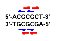
Figure 1: When using multiple methylation sites, the methylation patterns on the forward and reverse strands may differ. For the sequence ACGCGCT, all three dC residues could be methylated in a cell containing CG or GC methylation enzymes. The first and second dC residues are part of the CG recognition site (blue bar), while the second and third are in the GC site (red bar). However on the reverse complement strand (AGCGCGT), only two residues may be methylated and each site could be methylated by either enzyme.
Using MethylViewer
Getting started
Figure 2 Shows the main menu used to create an alignment or alter the alignment options.
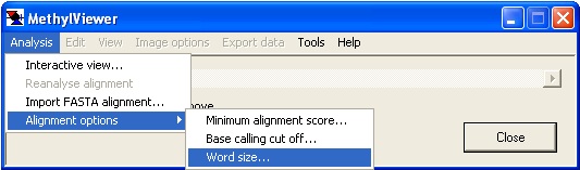
Figure 2
Alignment options
- Minimum alignment score:
- This sets the cut-off score at which a sequence alignment is accepted. The values range from 10 to 50, with a score of 10 roughly equating to 10% of the aligned sequence segments closely matching the reference sequence.
- Base calling cut off:
- This sets the minimum peak height at which the programme will call a nucleotide. This value is indicated by a red horizontal line across all electropherogram images. (See Figure 8b). This line should ordinarily be close to the bases of the trace peaks, unless the sequencing signal is very faint.
- Word size:
- This sets the initial size of a local alignment from which the global alignment is created. The valid range is between 6 and 15. The optimum value depends on the sequence of the specific DNA target region under study. Increasing the value reduces the overall alignment score, but may reduce the insertion of aberrant gaps (Figure 7).
Working with alignments
Data entry
Alignments can either be created by MethylViewer or imported from a pre-existing FASTA sequence alignment. In the latter case, the reference sequence must be the first aligned sequence in the FASTA file; this example file is a FASTA alignment in the correct format. These two options for creating an alignment are invoked respectively through the or the menu options. Selecting one of these options will invoke its corresponding data input form (Figure 3a or 3b). Rather than re-creating the same alignment multiple times, the option allows an existing alignment to be re-screened with a different set of methylation enzymes without re-extracting the underlying data from the trace files. Selecting this option invokes the methylation site input form shown in Figure 3c.
a 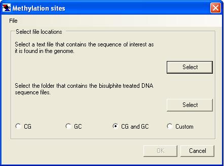
b 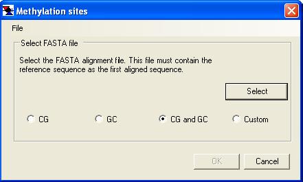
c 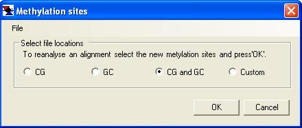
Figure 3: Data entry into MethylViewer. The two panels show the data input forms displayed when creating a new alignment (a) or importing a FASTA alignment created by another software package (b).
Both alignment options require the sequence data and a description of which methylation sites are to be analysed. When creating a new alignment, the programme requires a reference sequence file (plain text) and a folder containing the data files (Figure 3a), whereas only the single text file containing the alignment is needed when importing a FASTA alignment (Figure 3b). Once the data files have been selected, the methylation sites must be specified using one of the preset options (CG, GC, CG and GC, or Custom). If you routinely use the Custom option, your methylation site specification may be saved to file and re-imported each time a new analysis is performed. (To do this, first specify the custom sites (as described below) and then select from the form’s menu. To re-enter this site specification on a later occasion, select and pick the appropriate file.)
Specifying custom methylation sites
Selecting the Custom sites option invokes the Custom methylation sites window (Figure 4). When opened for the first time, this will already contain the sites CG and GC. If these are not required, they can be removed by selecting the relevant site from the list box below the button and then clicking . To add a new site, such as CpNpG, type its sequence in the upper left text box. The window will automatically display the site’s reverse complement sequence and the notional bisulphite-treated sequence in the lower two text boxes.
If the site contains a degenerate nucleotide, use the IUPAC 1-letter code abbreviations; these can be displayed by pressing the button. If the specified site contains more than one degenerate base (such as NCN), but not all possible combinations are used (e.g. if the first base is a purine, the third base must be a pyrimidine), tick the box beside any of the possible combinations that you do NOT want to use, displayed in the large text box.
Once you have entered the desired recognition sequence, specify which cytosine residue will be methylated by the enzyme, using the list located below the ‘Select the methylated dC residue on the forward strand’ label. Next, select a colour that you wish to use to specify this class of methylation site, again using the drop-down list of colours provided. In the example shown, the colour Lawngreen has been selected. Finally, chose the symbol that will be used to identify the site in exported images, by clicking on an icon at the bottom of the window. Each symbol may only be used once; symbols already assigned to other classes of site will be greyed out and unselectable.
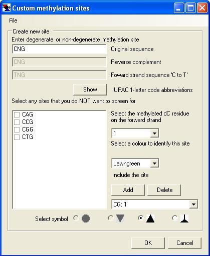
Figure 4: The Custom methylation sites form.
Viewing the data
The interactive grid view
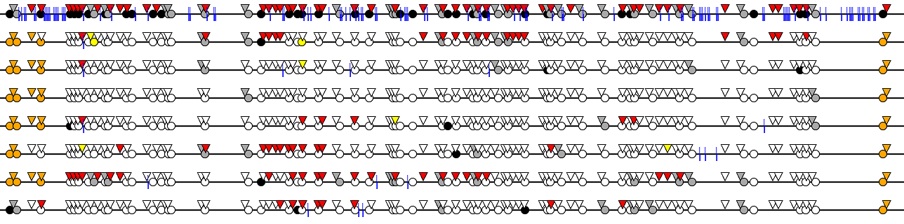
Once the sequence data and methylation sites have been selected, clicking the button will instruct MethylViewer to create and display the interactive grid (Figure 5). In this window, each methyltransferase recognition site is represented by a cell, which is colour-coded according to the status and sequence context of the methylatable cytosine within that particular query sequence (Table 2). (Alternatively, if the option (Figure 9) is deselected, all methylated residues will be shown as black cells.) When an alignment is created, the data grid is shown in a panel within the window. If the grid is too large for this panel, it can be scrolled horizontally using the slide bar at the bottom of the grid.
Regions of poor sequence alignment between the reference and bisulphite-treated DNA sequences are highlighted by a blue line; when this line is visible in a cell, it suggests the possibility that the methylation status may be incorrect at that site (This feature can be turned off by deselecting the option).
Moving the cursor over the grid invokes a small floating window next to the cursor, identifying the methylation site(s) represented by that cell. The information in this mini-window can be customized, via the menu, to show either the methylation consensus site or the actual sequence in the reference file these will be identical unless the recognition site is degenerate). For sites with more than one cytosine residue, the position of the methylated residue may also be displayed.
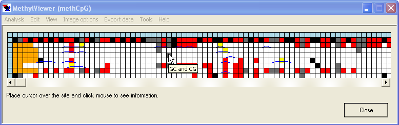
Figure 5: The interactive grid. Each square represents a methylation site and is colour-coded according to its methylation status (see Table 2).
| Colour | Status | Original methylation state |
|---|---|---|
| Orange | Not aligned in sequence. | Unknown |
| Yellow | The methylated residue is aligned to the reference sequence, but it is not possible to identify its methylation status. This could be due to poor sequence alignment, a sequencing artefact or a polymorphism between the reference sequence and the test DNA sample. | Unknown |
| White | dC converted to dT | Unmethylated |
| Pale blue | Special cell used to identify sequence information (see File and methylated cytosine identification below). | N/A |
| Grey | dC not converted, but could have been methylated by more than one enzyme | Methylated |
| Other colour | Unconverted dC residue that could only have been methylated by one enzyme. The colour matches the colour previously chosen to represent that recognition site. | Methylated |
Table 2: Colour codes and methylation status of cells in the interactive grid.
File and methylated cytosine identification
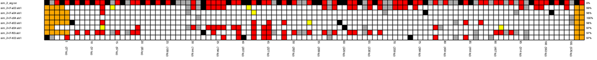
Selecting a grid cell by left-clicking causes that methylatable cytosine’s position in the reference sequence, its status within the query sequence and the query sequence's filename all to appear below the grid (Figure 6, highlighted in red). The blue squares forming the top and left edges of the grid can be used to access more detailed information about the methylatable cytosine (column headers) and the query sequence file (row leaders), again by left-clicking the square. Alternatively, right-clicking the blue square at the start of each row will open a window displaying the electropherogram trace image. The top left corner blue square contains statistics on the methylated cytosine status of the grid as a whole.
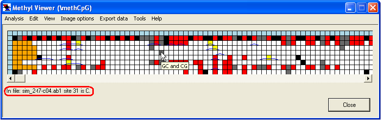
Figure 6: Left-clicking on the grid displays information about the methylatable cytosine represented by that cell.
Viewing the alignment
By right-clicking a square (other than the blue border and orange non-aligned cells), the underlying sequence alignment can be inspected. This can be either a global text alignment (plain text sequence files; Figure 7a) or a local section of this alignment along with the corresponding part of the electropherogram trace (Figure 8). In the latter case, the trace image will sometimes represent the reverse complement of the reference sequence. By default, the trace image is displayed, but by setting the option (Figure 9), the global (text) alignment will be displayed in preference. If it appears that inappropriate gaps have been inserted in the global alignment, increasing the Word size (via the ; Figure 2) may eliminate them (e.g. Figure 7a uses a word size of 6, compared to a word size of 10 in 7b).
a 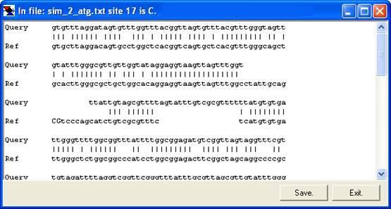
b 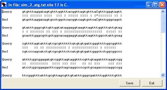
Figure 7: The underlying alignment can be displayed by right-clicking on a cell.
a 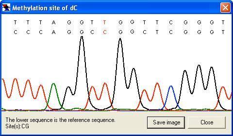
b 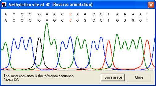
Figure 8: The alignment can be viewed as a section of the electropherogram (provided the sequence data originated from a trace file.) If the sequence read is in the reverse orientation to the reference sequence, the reverse complement of the latter will be shown (b).
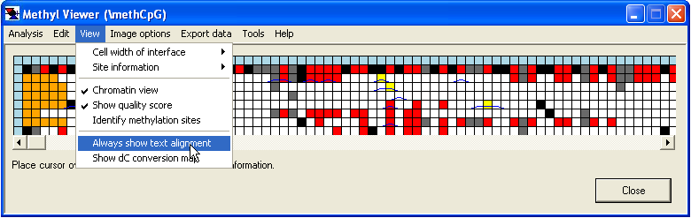
Figure 9: Selecting the Always show text alignment option forces MethylViewer to show the text alignment even for data originating from trace files.
Manual editing
Since bisulphite-treated DNA often contains long runs of low complexity sequence, the desired or correct alignment between modified sequence and reference sequence may not be the mathematically optimum one. In cases where the program miscalls a methylatable cytosine, it is possible to edit the methylation status of a cell. To edit the grid, select the option (Figure 10) and left-click the square to edit. This generates a floating menu that allows you to select the residue’s assigned status within the bisulphite-treated sequence (Figure 11).
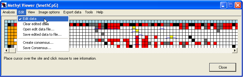
Figure 10: To manually edit the data, select the Edit > Edit data option.
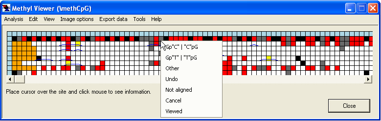
Figure 11: Left-clicking a cell creates a floating menu that allows the correct selection of the residue’s methylation status. If the residue could have been modified by more than one enzyme, all the recognition sites are shown.
The same floating menu can also be accessed by clicking the trace image or the text area of the global alignment window (Figure 12a,b), without the need first to select the option.
a 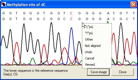
b 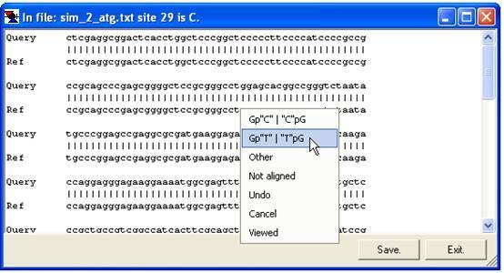
Figure 12: The floating Edit data menu can be accessed via the trace alignment window and the global text alignment window.
Squares that have been manually edited are identifiable; their new edited values are shown as smaller squares overlying the original image (Figure 13). With some limitations, the edited data can be saved to file or recovered from file, via the menu; however, this file contains only the editing information, and can only be used in conjunction with the correct reference sequence; individual sequence files may, however, be added or removed from the alignment.
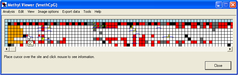
Figure 13: Manually edited cells have their corrected values shown as small squares within the cell. In addition, cells that have been examined but left unedited are identified by a still smaller green square.
Creating a consensus sequence
When several sequences are derived from a common source (e.g. multiple sequences from the same clone, or multiple clones from the same tissue sample), it may be desired to form a consensus sequence from them. Such a consensus sequence can also be re-loaded into the programme along with other consensus sequences, to form a grid that displays methylation status from multiple sequence files in an abridged manner. The option (Figure 14a) adds a new row to the bottom of the grid. The cells in this row are initially orange, but change to match whichever colour is chosen by clicking on any cell in the same column (Figure 14b). Once the consensus row is completed, the underlying sequence can be saved via (Figure 14a). If a square has been edited, the consensus sequence takes the colour of the edited value. Once a consensus has been saved, left-clicking the blue square at the start of the row clears the sequence. This allows multiple consensus sequences to be generated from a single alignment.
a 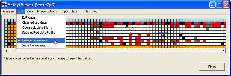
b 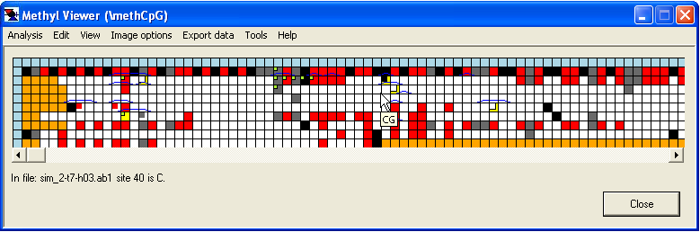
Figure 14: A consensus sequence can be produced by selecting Create consensus (a) and then clicking on a cell of the desired status (b).
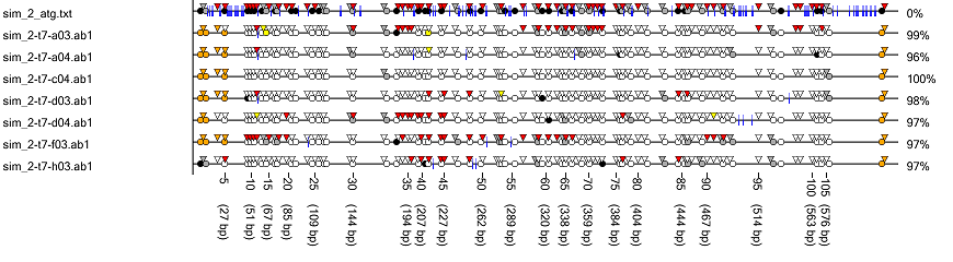
The dC conversion map
The efficiency of bisulphite modification of DNA is often not 100%, so that some unmethylated residues may remain unconverted. To identify sequences, which have low conversion efficiencies, it is possible to view the locations of unconverted residues in each sequence, by selecting the option (Figure 15). The data grid is now replaced by a map drawn to scale, that shows the positions of unconverted cytosine residues (blue vertical ticks) relative to the cytosine residues that lie within methylation recognition sites. The methylation status of the latter sites is colour-coded, orange for unaligned sites, black for methylated (residues within recognition sites), grey for unmethylated and yellow for status unknown. As with the interactive grid view, the underlying sequences can be viewed by left-clicking on the position of interest.
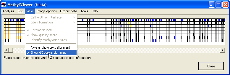
Figure 15: The dC conversion map identifies unconverted cytosine residues.
Saving grid data
Once an alignment has been created and edited, the grid may be saved, either as a text file or an image file, via the menu (Figure 16). If the option is selected (on the menu, Figure 17), the image will be generated from the edited grid; otherwise, the original methylation status will be used.
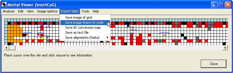
Figure 16: Data is exported via the Export data menu
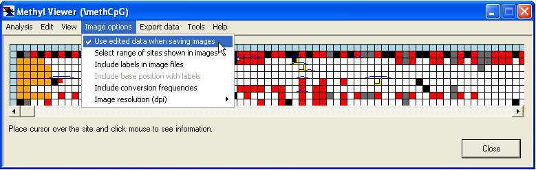
Figure 17: Edited data is used only if the Use edited data when saving images option is selected.
Image formats
The grid image and the dC conversion map image can be saved as bitmap (*.bmp), portable network graphics (*.png) or scalable vector graphics (*.svg) files. However, unlike CpGviewer, MethylViewer does not create PowerPoint presentation (*.ppt) files. The image file format is chosen when entering the image filename. In addition to the square pattern used for the screen display of the interactive grid, a “lollipop” style, as commonly used for publication, is available. Unlike CpGviewer, the symbols are spaced relative to the methylated residue’s absolute position in the sequence and are NOT shifted to reduce overlap and aid identification. This feature allows placement of footprints more accurately.
These exported images can be created unadorned or in an annotated format, which may include labels identifying the sequence file, nucleotide position of the cytosine residue(s) and the bisulphite conversion efficiencies. To add labels, select the appropriate option from the menu (Figure 17). It is also possible to trim the image, so that sites at the 5′ and 3′ ends of the alignment are not included in the exported ‘Grid’ or ‘Scaled Lollipop’ images.
To select a range of sites to export, use the option on the menu. This will invoke the corresponding Limit methylation sites shown in images window (Figure 18). This window allows the selection of methylation sites either by absolute nucleotide position or by order in the reference sequence. It is also possible to direct MethylViewer to renumber the exported sites, such that the start of the range for exported nucleotide position and methylation site number is reset to 1.
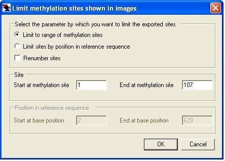
Figure 18: Methylation data included in exported image files can be limited to a specific range.
The symbols and colours used in the “scaled lollipop” image type correspond to those selected when defining the custom methylation sites (Figure 4). The position of the methylated residue is indicated by the position of the symbol in the image, as shown in Figure 19. For the triangular symbols, this is where the symbol touches the horizontal line. For the blue line (representing unconverted dC residues not within a recognition site) it is where the line bisects the horizontal line. In the case of the disc symbol, the residue position is at the left-hand edge of the disc where it intersects the horizontal line. In cases where a residue could be methylated by any of multiple enzymes, a symbol is coloured grey for methylated and white for unmethylated status. When creating the composite image (Figure 20), the various symbols will be drawn in the order in which they were specified in the Custom methylation sites. For this reason, if the disc symbol is used, it is suggested that this is defined first, since it may otherwise obscure other nearby symbols.
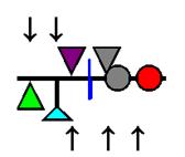
Figure 19: The positions of the methylated residues relative to their symbols are indicated by the arrows.
a

b
c

d
e
f

Figure 20: The methylation data can be exported as image files with (d-f) or without (a-c) annotation in one of three styles: the data grid (a,d), the “scaled lollipop” image (b,e) and the dC conversion map (c,f).
Text formats
It is possible to export the alignment data either as a tab-delimited text file representing the grid data, or as a FASTA alignment file. The FASTA file does not contain any information on methylation site locations, but allows the alignment information to be imported into other software packages.
Grid text file
This text file recreates the grid as a plain text tab-delimited table arranged in the same order as the grid, with each methylatable residue’s sequence replacing its colour-coded square. Each sequence is identified by the originating sequence file name at the end of the row. Since the table is tab-delimited, it can be conveniently opened using a spreadsheet programme, with each individual methylatable residue score placed in a cell. The '~~' symbol represents unaligned methylation sites. The file also includes the reference sequence, with the methylatable residues numbered in the order that they appear in the table. A key to these numbers is located at the end of the file which also identifies which recognition site contains the target residue (Figure 21). Note that the output to this file cannot be trimmed using the option (Figure 18).
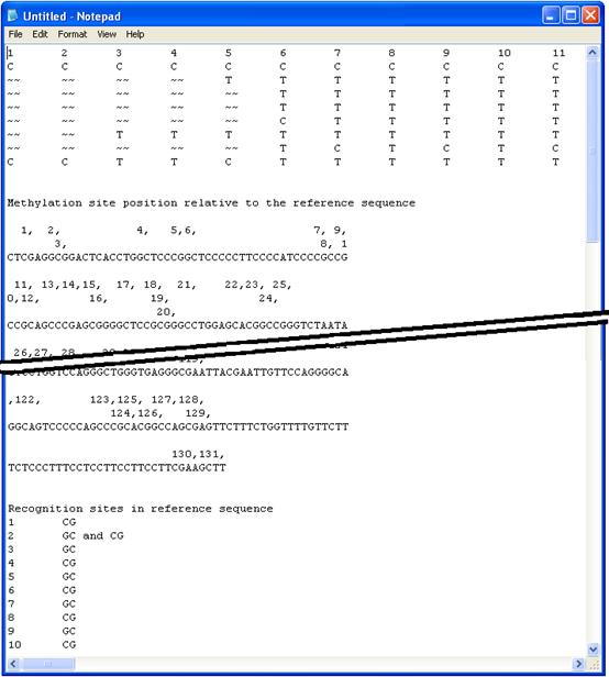
Figure 21: Data can be exported as a tab-delimited text file. This image is a composite that shows the both the data grid and the methylation site key.
FASTA text file
The FASTA text file can be created with or without the reference sequence. However, if you wish later to use the file with MethylViewer, it must include the reference sequence. For an example of a FASTA file, see here. The first sequence in the file must be the reference sequence, and gaps in the alignment must be identified by the '-' character.
Tools
MethylViewer also incorporates four other tools that may useful to researchers engaged in bisulphite genomic sequencing projects (Figure 22). These tools aid primer design, viewing of electropherogram data (view a trace) and creation of hypothetical bisulphite-modified sequences.
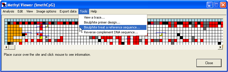
Figure 22: Additional tools.
Viewing an electropherogram
Sequence read electropherogram traces can be viewed either by right-clicking a blue square at the start of a row or by choosing from the menu and selecting a trace file. The trace will be displayed in a new window (Figure 23). If the selected file is an unprocessed ABI file (*.ab1), a message will be displayed stating that the file contains no processed data, and offering the choice either to view another file or allow the programme to analyse the data. Note that when unprocessed data is viewed (either from *.ab1 or *.rsd files) the display window will initially show the earliest scans from the run, which do not contain readable sequence data (Figure 24). The trace view can be altered or scrolled using the menu or the controls at the bottom of the window (Figure 25).
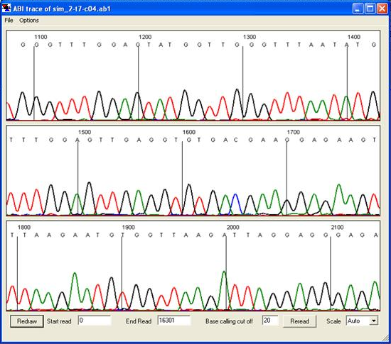
Figure 23: Electropherogram data can be viewed in the trace viewer window
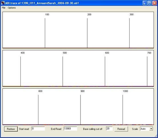
Figure 24: The start of an electropherogram may appear blank if it has not been base-called by the ABI base-caller.
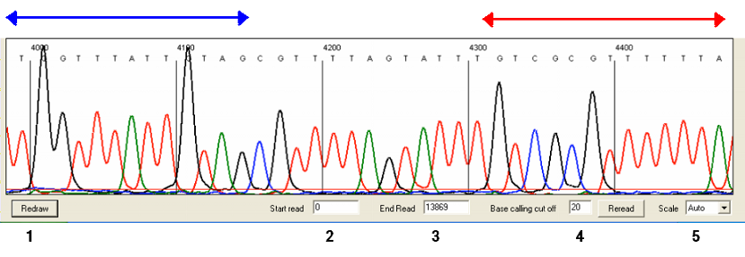
Figure 25: Clicking on the image in the region delimited by the blue and red arrows moves the sequence respectively 5′ and 3′ from its current position.
Navigation
The sequence trace is displayed as a series of panels, of which three are visible in the window. To view panels that contain data 3′ to the current view, left-click a panel in the region delimited by the red arrow (Figure 25); similarly, to move 5′ from the current sequence region, left-click in the region indicated by the blue arrow.
Saving the image
Each panel can be saved individually, as a bitmap, by right-clicking the image and choosing the file name and location. If the sequence of interest lies across two panels, adjust the start point of the images, as described below in Changing the start and end points of the images.
Changing the trace appearance
Applying changes
Since each change requires the images to be redrawn, to save time multiple adjustments can be made (as described below) and then applied using the or buttons (labeled in Figure 25). These buttons have similar functions, but differ in that whereas creates the new images using the existing data, recreates the basecalling and alignment to the reference sequence. If the base-calling cut-off is changed by a large amount, then it is preferable to use the button.
Changing the start and end points of the images
By default, all of a sequence run’s scan lines will be analysed by MethylViewer. To limit the range of scan lines used to create the images, enter the desired start and end points into the text boxes at the bottom of the screen (labeled 2 and 3 in Figure 25) and press .
Adjusting the base-calling cut-off
The base-calling cut-off (labelled 4 in Figure 25) adjusts the signal intensity at which peaks are identified as either true base-calls or background noise. With good quality sequences, this value is relatively unimportant, but it may be useful to adjust it when analysing traces that have low amplitude and/or high background. If changed, the cut-off value is stored by the programme and applied to all subsequent base-calling, whether displaying other traces or creating a methylation site alignment. The base-calling cut-off can also be adjusted via the menu of the main programme window (Figure 2).
Changing the image scale
The vertical scale can be adjusted via the list-box (labelled 5 in Figure 25), the new setting being applied once the button is clicked. If the scale is set to “Auto” the programme will use a suitable value calculated using the peak heights across the entire trace.
Changing the window size
The trace view window can be manually resized, but the trace image will not be redrawn to suit the new panel size until either the or button is pressed.
File menu functions
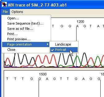
Figure 26 It is possible to open, save and print trace files using the menu.
Figure 26 shows the menu. Using this, it is possible to open a new trace file, save the sequence as a plain text file, or save the trace in standard chromatogram format (*.scf). The latter only includes scan data between the start and end values selected for creating the image (2 and 3 in Figure 25). This menu also allows the user to print the trace.
Options menu
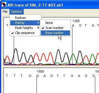
Figure 27 The format of the view panel is adjusted using the menu.
The menu (Figure 27) enables the user to change the format of the panels, as well as to access peak height data.
Available functions
- Redraw:
- this performs the same function as the button at the bottom of the form.
- Marker:
- This changes the marker intervals, to appear either every 10 nt or every 100 scan lines. It also allows the markers to be hidden.
- Peak heights:
- The average peak heights are calculated as the programme base-calls the trace file. This information can be shown either visually or as text. When the option is selected, horizontal lines are drawn to show the average peak height for each nucleotide. The option displays the average, standard deviation and count for each nucleotide.
- Clip sequence:
- This function removes the 3′- and 5′-end low quality sequence when it is saved to a plain text file.
Bisulphite primer design
Since the sister strands of bisulphite-treated DNA are no longer complementary, before designing primers it is necessary to select both the region of DNA sequence of interest (plain text file) and which strand the user wishes to analyse (Figure 28). It is also possible to have CG and/or GC methylation sites highlighted on screen when designing the primers.
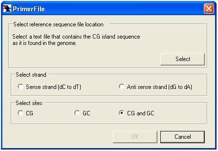
Figure 28
The primers are then designed using the primer design window (Figure 29), which comprises four parts, as described below.
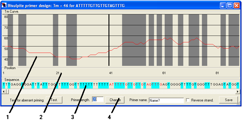
Figure 29
- 1. The Tm graph.
- This shows the Tm of a primer starting at that position and extending to the right by the length entered in the Primer length box. The solid black vertical line shows the start point of the current primer. The grey boxes show the positions of methylatable sites (CG and/or GC) in the reference sequence.
- 2. The position panel.
- This panel shows the position (in base-pairs) of the sequence in the Tm graph and sequence panels.
- 3. The sequence panel.
- The predicted sequence of the bisulphite-treated DNA reference sequence if unmethylated. Pale blue boxes indicate where dC residues have been converted to dT, and the red text represents the current primer sequence.
- 4. The function panel.
- This region contains the controls used to create the primers.
How to design a primer
1. First enter the desired primer length in the Primer length number box and click . This redraws the Tm graph shown in the main panel (the primer length can be changed at any point during the primer design process).
2. Navigate to the desired region in the DNA sequence, using the scroll bar across the top of the function region, and choose a suitable point in the sequence.
3. If this is the reverse primer, tick the Reverse strand box.
4. Click the point at which you wish the primer to start (forward primer) or end (reverse primer) on the Tm graph panel, the position panel or the sequence panel. The primer sequence will be highlighted in red text in the sequence panel and will be displayed in the window’s title bar, along with its calculated Tm. The Tm is calculated using Tm = 81.5oC + 16.6oC x log10[positive ion conc] + 0.41oC x (%GC) - 675/primer length. The positive ion concentration constant is derived from the standard Promega PCR buffer containing 1.5mM MgCl2 (Sambrook, J., Fritsch, E.F. and Maniatis, T. (1989) Molecular Cloning: A Laboratory Manual, Cold Spring Harbor Laboratory Press, Cold Spring Harbor, NY.). If the Reverse strand box is ticked, the complementary sequence appears in the title bar (but not in the sequence panel).
5. Pressing the button (bottom left of the function panel) displays a text field with information on possible problems that may arise with the chosen primer, from primer self-annealling and positions of (ungapped) homology along the DNA sequence.
6. Enter the primer name in the relevant text box and press . When prompted for a filename, if a new filename is entered, a plain text file will be created, while if an existing file is chosen, the new primer will be appended to that file. The primer is saved as tab-delimited plain text, as shown in Table 3.
| Column 1 | Column 2 | Column 3 | Column 4 | Column 5 | Column 6 |
|---|---|---|---|---|---|
| CpG1R | Starting at: 367 | Primer length: 20 | Tm: 46 | Reverse direction | CCACAAAAAA AACACTAAAA |
| CpG1F | Starting at: 71 | Primer length: 20 | Tm: 52 | Forward direction | AGGAGGTAAG TTAGTTTGGT |
Table 3
Hypothetical bisulphite-modified sequences
In common with CpGviewer, MethylViewer also allows the user to generate the predicted sequences of bisulphite-modified DNA molecules. Note that these sequences must not be used as reference sequences for MethylViewer. For the CG methylation site, it is possible to specify the methylation state prior to performing the in silico bisulphite modification.
To generate a bisulphite-modified sequence, select the option (Figure 22). This causes the form shown in Figure 30 to be displayed. The user must then load the DNA reference sequence (as a plain text file) and choose the methylation status of the DNA (methylated or unmethylated at CG residues; other dC residues always assumed to be unmethylated) and whether the forward (dC to dT) or reverse (dG to dA) strand is to be created. Pressing prompts the user for a file name and then saves the modified sequence to the file.
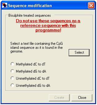
Figure 30
Reverse complement a DNA sequence
Since MethylViewer will no longer align sequence to the forward and reverse complement sister strands, it may be necessary to reverse complement the reference sequence. To reverse a reference sequence, select the option (Figure 22) and select a plain text file containing the reference sequence. Finally, enter the name of the output file that will contain the reverse complement sequence.