Appendix
Back to the user guide
Construction of the curves used in the Raw data and Normalise views
The DNA melting data actually undergo a number of manipulations before being displayed as Raw data. Figure a1 shows the initial graph of fluorescence (y axis) against temperature (x axis). (The thick blue line represents the data from a well containing no DNA.) The fluorescence data for each temperature point is first recalculated, as a percentage of that sample’s maximum fluorescence (Figure a2). These data are then scaled, such that each curve has a final value of zero while maintaining an initial value of 100 (Figure a3). These data are then used to derive a graph that shows rate of change of fluorescence relative to temperature (dF/dT, actually approximated by dF/dT for each time increment) plotted against temperature (Figure a4).
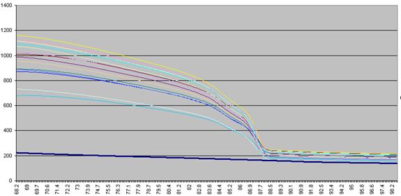
Figure a1: Raw fluorescence data from the LightScanner containing 92 samples and 1 blank (thick blue line: no DNA).
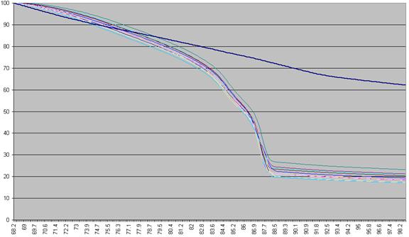
Figure a2: Fluorescence data as seen in Figure a1 shown as a percentage of each sample’s first reading.
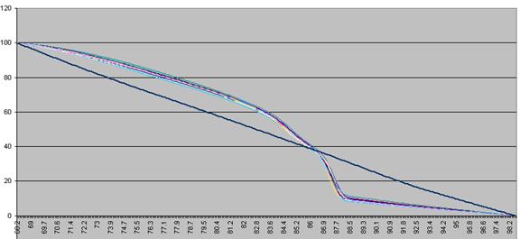
Figure a3: Fluorescence data shown in Figure 8 adjusted so that each curve ends with a value of zero.
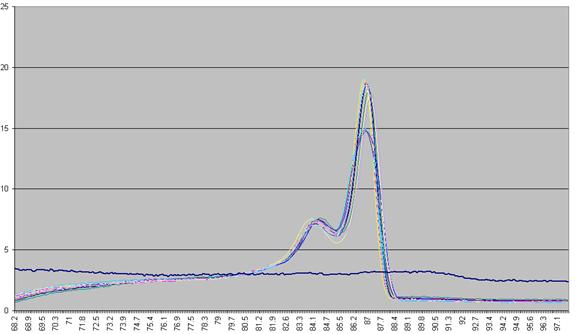
Figure a4: Graph plotting the (-) rate of change in fluorescence (-dF/dT) against temperature.
The vertical displacement of this derivative curve varies, depending on the temperature range over which the readings are taken. To standardise this displacement, the average gradient across the whole temperature range is subtracted from the data (Figure a5). This is equivalent to subtracting an idealised blank from each curve; the “experimental” blank (blue line in Figure a5) can be seen to lie close to this zero line.
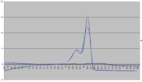
Figure a5: Graph showing -dF/dT against temperature with a standardised cut-off.
The graph in Figure a5 shows two pronounced peaks at approximately 84.3oC and 87oC. These peaks can be seen to match the regions in Figures a1-a3 where the gradient of the graph is steep, representing two successive domains melting. The present programme is designed to analyse DNA products with up to three distinct domains. If a curve contains more points it is not drawn and is flagged as "non-wildtype".
Construction of the data points used in the Peaks view
In order to define the data points, the programme scans along the fluorescence data, looking alternately for peaks and troughs. When it has completed this task, it returns to the first peak, and scans backward to find the point at which the dF/dT value increases above the cut-off value (or 0). Once a peak or trough is found, the surrounding data points are examined to decide if the true minimum or maximum value lies between two consecutive temperature readings; if so the point is moved along the temperature axis to correct for the semi-quantitative nature of the readings. If a peak and a trough are very close together (i.e. within 3 temperature readings) the programme will miss the trough and ignore the next peak. Curves that exhibit this feature may still be correctly analysed by eye, but should not be considered for automatic analysis.
These data points are grouped into clusters corresponding to their positions, as shown in Figure a6. It is the position of each data point relative to these clusters that is assessed in order to assign the genotype of a sample. If all the data points defined for a curve lie within the chosen statistical limits of their respective clusters, then that curve is considered to represent a wildtype genotype. If a curve does not contain all three clusters then the empty cluster points are ignored.
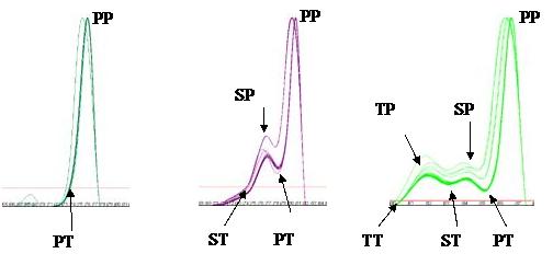
Figure a6: Naming of the peak and trough data points. (PP = primary peak, PT = primary trough, SP = secondary peak, ST = secondary trough, TP = tertiary peak and TT = tertiary trough).
Locating a cluster’s position and size
To permit analysis of data points, the position of the relevant cluster must be defined. This can either be done statistically, or by the use of known control DNA samples. If no controls are set, all the sample data points for the cluster are calculated and then their median value is set as the cluster’s centre point. Alternatively, if control samples are used, then the centre point for the cluster is set to the arithmetic mean position of the control samples’ data points. A red circle highlights the cluster’s centre point (Figure a7).
Once the cluster’s centre has been defined, the spread about that point is calculated as an average absolute deviation (AAD) value from that point. Then, a chosen number of AADs is used to define a window, within which individual data points must lie to be scored as normal. The number of AADs to be used for this window depends on the intra-assay variability and the target DNA’s profile. It can be set using the Temperature and dF/dT options of the Stringency submenu ( > > or ). The stringency can be independently set for the x and y axes. (The actual AAD value used is derived from a second calculation, after excluding outliers; in other words, the AAD is initially calculated from all data points; points outside the cutoff range are then discarded and the remaining data points used to recalculate the AAD, which is then used to assign points as inside or outside the final cut-off window.)
If control samples are used, then it is possible to set the distribution for the x and y axes via the Plate setup window. When the option is selected, the and text boxes are enabled. If non-zero numbers are entered, then these are used instead of the calculated MAD values. Unlike the MAD values, which vary between clusters, this distribution is the same for each cluster.
The limits of the cluster are shown in the Peaks view as a box around the clustered data points. Each cluster has a unique colour that is shared between the data points, the box showing its limits and any shoulder that may be related to the cluster (Figure a7).
Determining the genotype of a sample
Once a cluster’s size and location are determined, it is possible to score each sample as either wildtype or not. If a curve contains any data point which falls outside the boundary of its correscponding cluster, that sample is scored as non-wildtype, whereas curves that have all of their data points within the appropriate clusters are scored as wildtype.
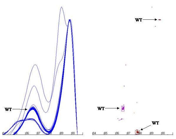
Figure a7: Demonstration of the programme’s ability to identify and size the clusters related to the wildtype genotype and exclude data from non-wildtype samples
Last modified: Wed, 15th Apr 2020, at 10:53 pm