User guide
Introduction
AgileGenotyper determines genotypes for over 0.5 million SNPs that have been identified by the 1000 Genomes Project and are located in protein-coding exons or their closely flanking intron sequences. The analysis is performed in the same manner as AgileAnnotator, except that AgileGenotyper only genotypes specific positions known to be polymorphic, then comparing the deduced genotype to the known alleles. If the deduced genotype is consistent with the known alleles, it is stored. However, if the deduced genotype includes unknown alleles, or the position cannot be called for reasons of read depth, the position is recorded as a “No-call”. Triallelic or indel variants are not genotyped.
Compared to AgileAnnotator, the default read depth and minimum minor allele frequency required by AgileGenotyper are more stringent, with a minimum read depth set at 7 reads for the two most common alleles at a given position. A position is called as heterozygous if 25% or more of the reads identify the minor allele. Table 1 highlights the variant-calling criteria:
Genotyping criteria, by example
| A | C | G | T | Read depth (minor+major) | % minor allele | Comments |
|---|---|---|---|---|---|---|
| 0 | 0 | 0 | 6 | 6 | 0% | No-call, since read depth <7 |
| 0 | 0 | 0 | 7 | 7 | 0% | Homozygous |
| 2 | 0 | 0 | 5 | 7 | 28.6% | Heterozygous A/T, as minor allele is >25% of major+minor allele read depth |
| 1 | 1 | 0 | 5 | 4 | 25% | No-call, as combined read depth <7 for major and a single minor allele. |
| 1 | 4 | 1 | 7 | 11 | 36% | No-call, as minor allele read depth is not more than twice the read depth of the remaining two (presumptively erroneous) bases (A+G) |
| 0 | 25 | 0 | 75 | 100 | 25% | Heterozygous A/T, since minor allele is 25% of major+minor allele read depth |
| 0 | 25 | 0 | 76 | 101 | 24.7% | Homozygous T, since minor allele is <25% of major+minor allele read depth |
| 0 | 25 | 0 | 74 | 99 | 25.2% | Heterozygous A/T, since minor allele is >25% of major+minor allele read depth |
| 0 | 25 | 10 | 75 | 100 | 25% | Heterozygous A/T, since minor allele is 25% of major+minor allele read depth |
Table 1
Creating an annotation file
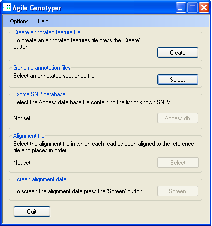
Figure 1: AgileGenotyper user interface
AgileGenotyper is designed to derive genotype information from exome pulldown sequence data. In keeping with this aim, AgileGenotyper refers to an annotation file that contains the locations of protein-coding exons and their genomic sequences. This file can be created by either AgileGenotyper itself or the related program AgileAnnotator. To create an annotation file, press in the Create annotated feature file panel (Figure 1). This causes the Annotation file creation window to be displayed (Figure 2).
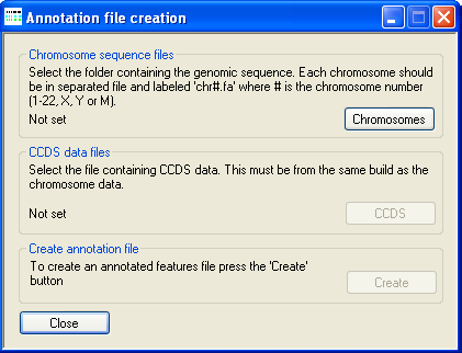
Figure 2: The annotation file creation window
The positions of the SNPs in the Access™ database are defined relative to the hg19 reference sequence build; therefore, the genomic sequences in the annotation files and the CCDS data file MUST both be derived from the hg19 build. If discordant reference sequences are used, the analysis will fail!
The location of the uncompressed FASTA-format genomic reference files is selected using the button under Chromosome sequence files. These reference sequence files must follow the specific naming convention where each file name starts with "chr" followed by either the chromosome number or "X" or "Y", and has the .fa file extension. Permitted names include chr1.fa, chr5.fa for an autosome, while the X and Y may be named chrX.fa or chr23.fa and chrY.fa or chr24.fa, respectively. (Note that while it is possible to include Y chromosome data in the annotation file, the Access™ database does not contain any Y-specific SNPs. Most other programs designed to handle SNP genotype data also ignore the Y chromosome.)
Next press the button in the CCDS data files panel and select the file containing the positions of the coding sequences as described by the Consensus CDS (CCDS) project. These files can be downloaded from the NCBI CCDS web page or FTP site.
Finally, press the button under Create annotation file and enter a name for the genomic annotation file. Since AgileAnnotator has to read all of the sequences in the genomic reference files and then write a large amount of data, the creation of the annotation file may take several minutes.
Genotyping an exome-derived SAM file
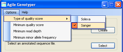
Figure 3: Adjusting the variant calling parameters
Before a SAM file is screened for sequence variants, it is necessary to select Solexa- or Sanger-type quality scores, using the option, and to adjust the variant calling cut-off parameters (quality and read depth), all accessible under the menu (Figure 3).
Figure 4: Entering data
Once the analysis cut-off parameters have been set, press the button in the Exome SNP database panel (Figure 4) and select the database file containing the SNP genotype and position data (download here). Note that while this file is an Access™ database, it is not necessary to have the Microsoft Access™ program installed on the computer.
To select an ORDERED SAM file, press Alignment file → (Figure 4) and enter the name of the SAM file to be genotyped. The aligned sequence reads in this file must be ordered by chromosome and chromosomal position. Finally, press Screen alignment data → (Figure 4) and enter the name of the file to save the genotype data to. AgileGenotyper will then export the SNP genotypes as it reads the SAM file, showing the progress of the analysis in its title bar (Figure 5). Since AgileGenotyper only stores the sequence reads for one gene at a time, it is not memory-hungry, and the speed of the analysis is limited by the speed at which it can read the SAM file (which should therefore be stored on a local hard drive).
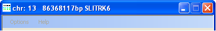
Figure 5: The title bar of AgileGenotyper shows the status of the analysis.
Analysis of data produced by AgileGenotyper.
The data exported by AgileGenotyper can be directly imported into AutoSNPa and compared to other data files generated by AgileGenotyper. However, if the exome-derived data are to be used in conjunction with genotypes of a different set of SNPs (e.g. from a SNP microarray), IBDFinder should be used instead. If the data are difficult to analyse due to an excess of spuriously heterozygous calls, one option may be to re-genotype the variants using AgileVariantMapper.
Comparison of exome-derived SNP data with SNP microarray data
Exome-derived SNP data differ from commercial SNP microarray data (e.g. Affymetrix Axiom) in two important ways. Firstly, in a typical SNP microarray, a quarter to a third of the SNPs will be heterozygous. In contrast, we observe that less than 4% of SNPs derived from an exome sequencing experiment are heterozygous (and <2.5% of SNPs are homozygous for the non-reference allele). This means that only about 25,000 SNPs from an exome will differ from the reference sequence. Secondly, coverage of a region by exome-derived SNPs is strongly affected by the local gene density. Consequently, in some regions of the genome, small-scale features (<4 Mb) cannot be accurately identified. Figure 6 shows a comparison of exome-derived data (lanes 1 to 3) against Affymetrix Axiom microarray data (lane 4), for Chrs. 1, 5, 10, 11 and 13. In each case, the exome genotypes were extracted using a minimum quality score of 10, read depth of 7 and minor allele frequency of 10%, 25% or 40% (lanes 1, 2, 3 respectively). While many autozygous regions (red bars) can be identified in the exome data, microarray data generally perform better for this purpose. Figure 6D, for example, shows two regions of autozygosity that are not detectable in the exome data, because they contain very few coding sequences and hence few sequence variants. Similarly, Figure 6E shows data for Chromosome 13; an extended region of low gene density is revealed by its very low SNP coverage, which would make this region very difficult to assess for autozygosity.
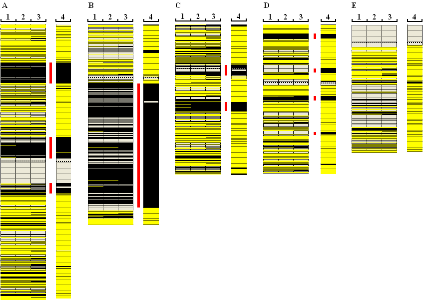
Figure 6: A comparison of exome-derived SNP genotyping data against Affymetrix Axiom microarray data. Figures A to E represent Chromosomes 1, 5, 10, 11 and 13 respectively. The minor allele frequency cut-off value was 10%, 25% and 40% for lanes 1 , 2 and 3 respectively. The red bars show regions of autozygosity.