User guide
Introduction
This program is designed to identify the haplotype of PCR products which contain a number of polymorphic positions, such as those that amplify the exons of the immunoglobin proteins. If a set of known alleles is imported, HaplotypeViewer will compare the genotype of each sample and attempt to identify which combination of alleles could be present in the sample and so deduce the samples haplotype.
Entering data
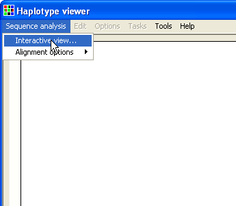
Figure 1 |
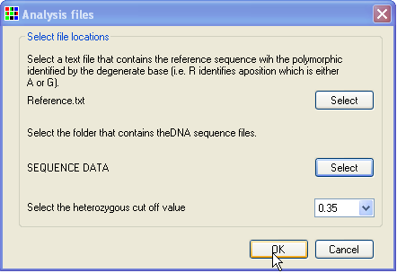
Figure 2 |
To enter your data, select the > menu item (Figure 1). Then, enter your reference sequence as a text file, with the known polymorphic positions marked using the IUPAC ambiguity symbols (Y, R, W, S etc). Do this by pressing the upper button (Figure 2). Next, press the lower button and pick the folder that contains the test sequence files. (The folder that contains the reference file will be selected by default.) Finally, press and HaplotypeViewer will align the sequence data to the reference sequence and identify the nucleotide sequence at each polymorphic position.
Checking the data
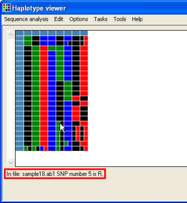
Figure 3
The data is displayed as a grid, with each test file shown as a row and each column representing a polymorphic position. The first row and column are composed of blue cells which contain information about the sequence file for that row or polymorphic position for that column. The rest of the cells identify the nucleotide sequence in the relevant file and polymorphic position. These are colour coded so that green is dA, blue is dC, black is dG and dT is red. Homozygous positions are uniformly coloured squares, while heterozygous positions are split into two differently coloured rectangles. If larger than the window, the grid can be scrolled using the scroll bars flanking it. To see this information (as text), place the cursor over the cell and read the text at the bottom left of the window (highlighted by the red rectangle in Figure 3).
Visualizing the underlying data
There are two ways to visualize the sequence data underlying the grid cells:
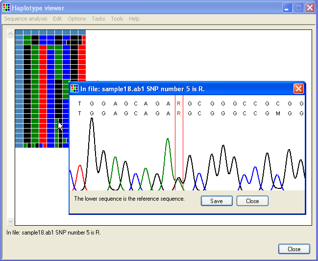
Figure 4
To view a single position, click the right mouse button when the cursor is over a cell. A window will appear that shows the electropherogram around the chosen polymorphic position; the selected residue is shown between two red lines (Figure 4). The image contains two DNA sequences as text; the upper line is the sequence in the trace file, while the lower line represents the sequence in the reference file. To view a different position, you must now close this window.
Alternatively, to rapidly view a number of grid positions, select the > menu item. This opens a window like the one in Figure 4, but now, as you move the mouse over the grid, the image in this window will be updated automatically.
Irrespective of the path taken to create this window, the information corresponding to the current SNP is shown in the title bar and if the sequence is the opposite orientation to the reference sequence, the phrase "Reverse orientation" appears in the lower left corner of the form. However, the electropherogram image is always drawn so the reference sequence is shown in the same orientation as it is in the reference file.
Viewing the sequence alignment as text
Selecting > and then clicking a cell opens a window that shows the sequence alignment for that sequence file, with the relevant position highlighted by an asterisk (highlighted by the red rectangle in Figure 5). To see an entire electropherogram, either right-click the blue cell at the start of the row or select > and navigate to the file (Figure 6).
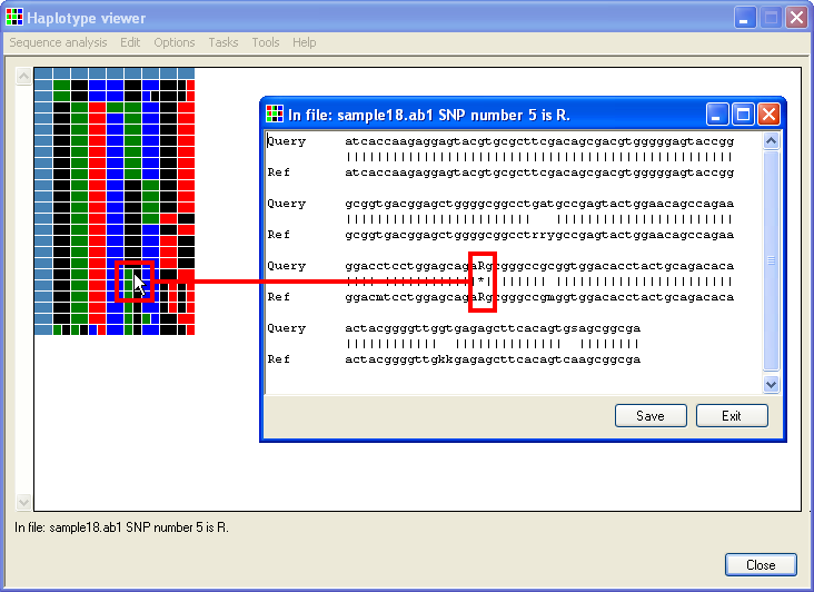
Figure 5
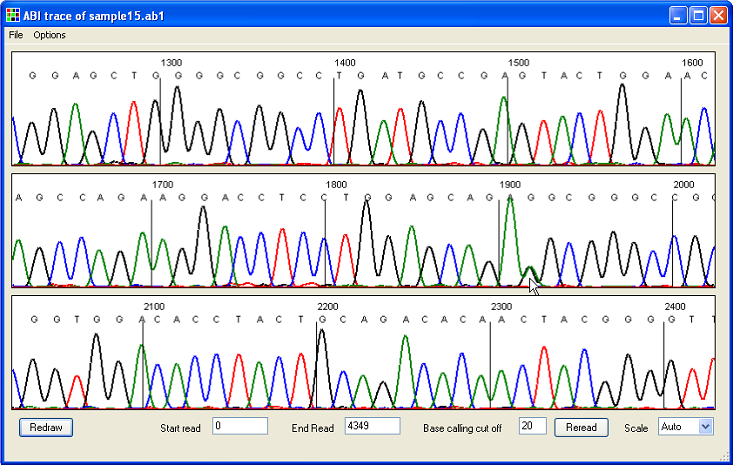
Figure 6
Editing data
It is possible to edit the displayed data via a floating menu, which can be invoked in various ways; if either of the windows shown in Figure 4 or 5 is displayed as a result of clicking on the grid, then clicking on the sequence's image or text alignment reveals the floating menu (Figures 7, 8). Alternatively, if the option is selected, clicking on the grid using the right-hand mouse button will display the floating context menu (Figure 9).
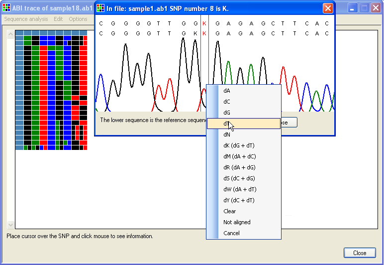
Figure 7
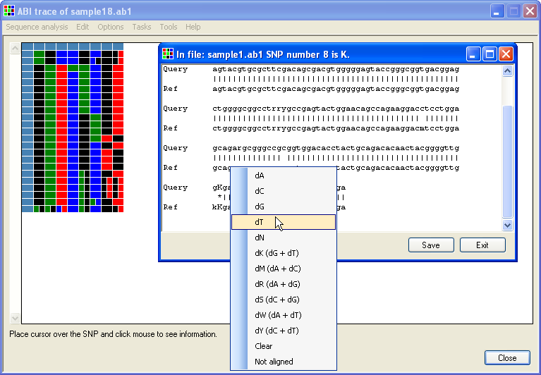
Figure 8
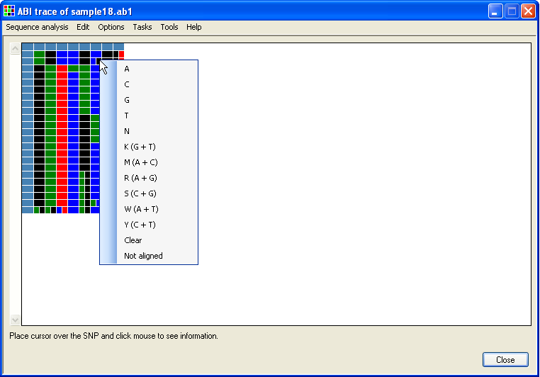
Figure 9
Selecting a different nucleotide sequence using the floating menu item modifies both the underlying data and the data grid to match the selected genotype. To highlight modified positions, the end genotype is displayed as a smaller cell overlying the original genotype (Figure 10).

Figure 10
Exporting data
Data can be exported as an image or as text as described below. By default, the exported data includes any editing that has been performed. To save the unedited data select the option and deselect it.
Exporting haplotype data as text
When exported as a text file, the data for each trace file is organised as a grid with the columns representing a single polymorphic position and each row containing data from a single trace file. The order of the trace files is sorted by the alphabetical order of their genotypes. It is possible to save the data with or without a list of the possible haplotypes present in each sample (Figure 12 and 14). To export the data without a list of possible haplotypes, simply select the the option and enter the name of the file to save the data in (Figure 11).
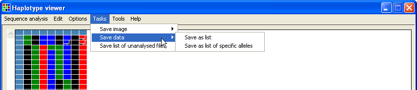
Figure 11
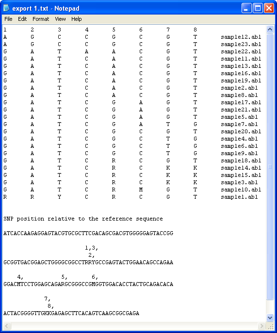
Figure 12
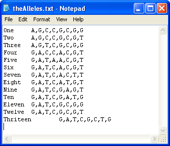
Figure 13
To save the data with a list of possible haplotypes, it is first necessary to create a file that contains a list of the known haplotypes linked to the reference sequence. The format of this file is shown in Figure 13 and can be created either manually or by using the Haplotype file construction function of HaplotypeViewer (see below). Each row in the file contains the name of the allele, a 'tab' character and then a comma delimited list of the nucleotides at each polymorphic position.
To save the data with a list of possible haplotypes select the option (Figure 11), select the file of known alleles linked to the reference sequence and finally enter the name of the file to export the data too. The format of the exported data is shown in Figure 14, with the first column of the file containing a list of possible haplotypes combinations that the sample could contain. If the sample is homozygous and contains a allele in the imported list the name of the allele is given in this column, but if the sample's haplotype was not found in the list the term 'Unknown' is placed in this column. If a sample is heterozygous and could be the result of two known alleles, the names of the alleles are listed, if it is possible that more than 1 combination of alleles could result in the samples haplotype, then each of the possible combinations is listed. If the sample is heterozygous, but HaplotypeViewer could not identify two alleles that could create the haplotype, a list of alleles that could be present in the sample is given followed by the word 'Plus'.
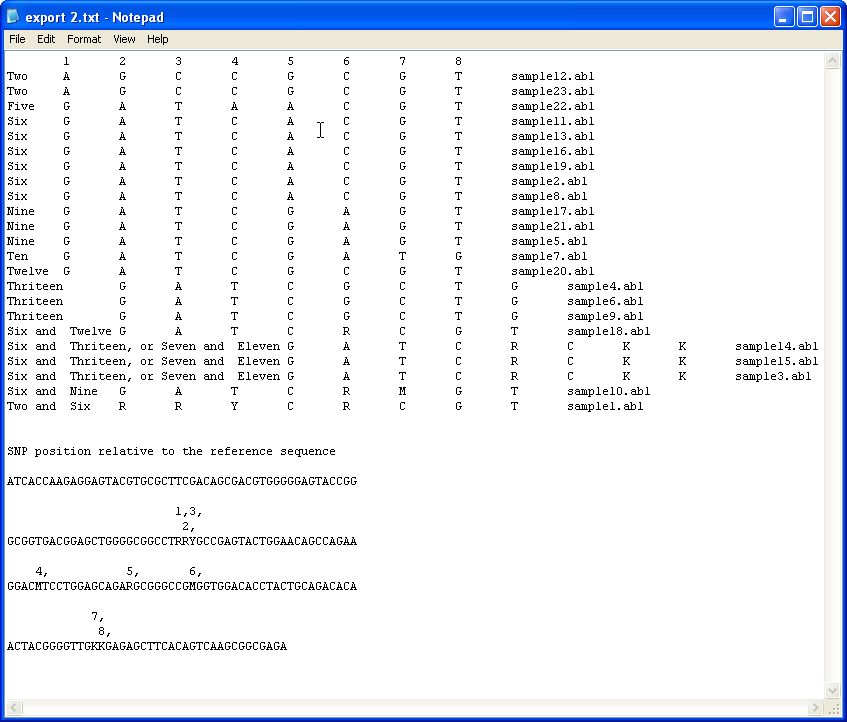
Figure 14
creating a file of known alleles
While it is possible to manually create a file containing a list of known allele, the file can also be created by HaplotypeViewer via the Haplotype file construction function (Figure 15).
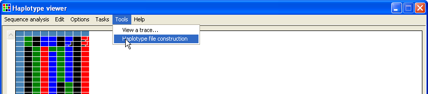
Figure 15
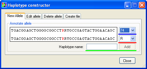
Figure 16
When this menu option is selected HaplotypeViewer prompts the user to select a text file containing the reference sequence, in which the polymorphic positions are marked using the IUPAC ambiguity symbols (Y, R, W, S etc) before opening the Haplotype constructor window (Figure 16). This window contains four tabs: , , and . To create a new allele select the tab (Figure 16). Each polymorphic position is entered by selecting its position in the reference sequence using the list of positions (underlined by the blue line in Figure 16) and then selecting the appropriate base from the list (underlined by the red line in Figure 16). As the nucleotide at each polymorphic position is selected the position is highlighted in red in the Annotate allele panel, with the lower sequence changed to reflect the current nucleotide selection. Once an allele has been created, it can be stored by entering a suitable unique name in the text box and pressing the button (underlined by the green line in Figure 16).
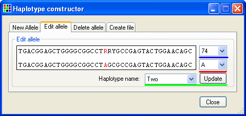
Figure 17
To edit a previously stored allele, select the tab (Figure 17) and select the name of the allele from the list of allele names (underlined by the green line in Figure 17). Then select the appropriate position from the list of polymorphic positions (underlined by the blue line in Figure 17) and edit the position's sequence using the list of available nucleotides (underlined by the red line in Figure 17) and finally save the changes by pressing the button (underlined by the green line in Figure 17)
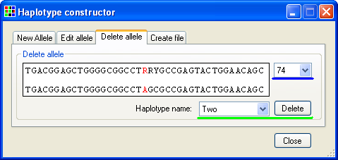
Figure 18
To delete a stored allele, select the tab (Figure 18) and select the name of the allele from the list of allele names (underlined by the green line in Figure 18) and then press the button. While it is not possible to modify the sequence of an allele in the tab, it is possible to observe the genotype of the polymorphic positions by selecting a position from the list of polymorphic positions (underlined by the blue line in Figure 18).
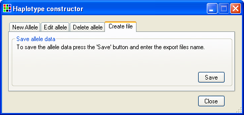
Figure 19
To save the stored alleles to a text file select the tab (Figure 19) and press the button.
Exporting data as an image
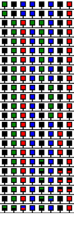
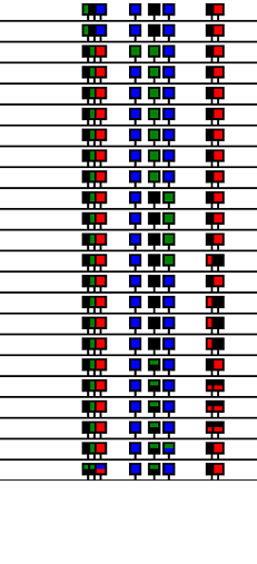
Data can be exported in any of three image styles (Figure 21a - f) by selecting the appropriate option in the menu (Figure 20). To include labels in an image, select the > option (Figures 21b, d and f).
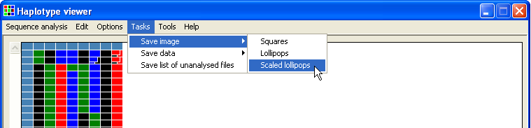
Figure 20
| A | B |
 |
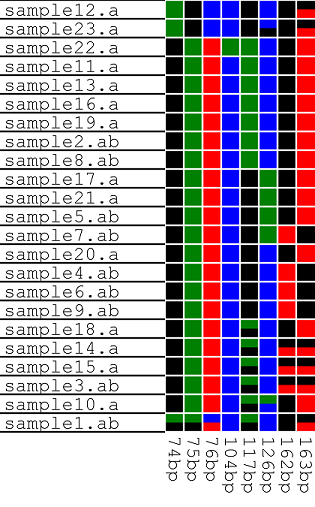 |
| The option arranges the data as a grid, each column represents a polymorphic position, while each row contains data from a single trace file. Heterozygous positions are shown as squares containing two colours. | |
| C | D |
 |
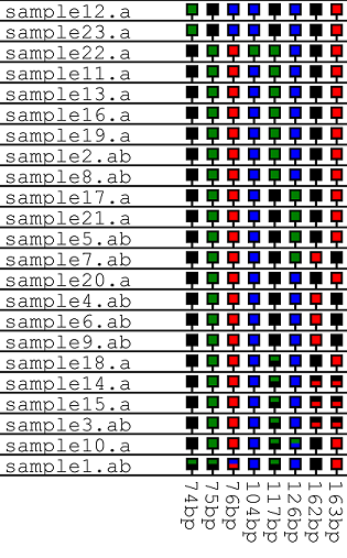 |
| The option arranges the data as an unscaled grid of 'lollipop' icons, each column represents a polymorphic position, while each row contains data from a single trace file. Heterozygous positions are shown as icons containing two colours. | |
| E | F |
 |
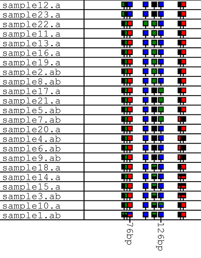 |
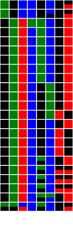
| The option arranges the data as an row of 'lollipop' icons with the icons positions on the horizontal line reflecting its position in the reference sequence. The order of the icons represents the order of the polymorphic position in the reference sequence, while each row contains data from a single trace file. Heterozygous positions are shown as icons containing two colours. | |
Figure 21